In the previous section we saw that for second-order systems, PD
control could be used to exactly specify the pole location of the
closed-loop system. This chapter examines the design problem of how to
select the pole locations to achieve desired
behavior. In
Section 11.1.1 we derive the
relationship between a single pole location and the step
response of the system. In
Section 11.1.2 we show that the
time-domain response for a second-order system can be understood in
terms of natural frequency and damping
ratio. Finally, in
Section 11.1.3 we show the effect that
a zero has on the step response of a second-order system.
8.1.1 First Order Response
Consider a first-order system given by \[Y(s) = \frac{p}{s+p} U(s),\] where \(p>0\). The pole location of the
first-order system is at \(-p\). If
\(U(s)=\frac{A}{s}\) is a step of
magnitude \(A\), then \[Y(s) = \frac{Ap}{s(s+p)}.\] As shown in
Appendix 29, the inverse Laplace
transform is given by \[\tag{8.1}
y(t) = \begin{cases} A(1-e^{-pt}), & t\geq 0 \\ 0, &
\text{otherwise} \end{cases}.\] The response is shown in
Fig.8.1,
which shows the response to steps of size \(A=1\), \(A=2\), and \(A=3\), respectively.
Interactive Figure 8.I1
First-order step response
Adjust the pole location p and the step magnitudes A to see how
y(t)=A(1-e-pt) changes. The 90 percent rise time is
independent of A, but the initial slope is A p.
Interactive
Figure 8.I1. Step response of a first-order system with pole parameter p
and step magnitude A. The step magnitude changes the final value and
initial slope, while the normalized 90 percent rise time is set by
p.
Live response values
Pole
Rise time
Initial slope
If we define the rise time \(t_r\) of the system to be the time after
the step when the response reaches 90% of its final value, then we note
from
Fig.8.1
that the rise time is independent of the step size \(A\). Also, by differentiating
Equation 8.1
at time \(t=0\), it is straightforward
to show that the slope of the response at \(t=0\) is equal to \(Ap\). This is also shown graphically in
Fig.8.1.
When \(A=1\), the step response for
different pole locations is shown in
Fig.8.2.
Pole locations corresponding to \(p=1\), \(p=2\), and \(p=4\) are shown. Note that as the pole
location moves further into the left half of the complex plane, the rise
time decreases.
Figure 8.2.
Interactive step response of a first-order system. Use the slider to
vary pole location (p); larger (p) values move the pole further left and
produce a faster rise time.
An important concept for the steady-state response of a system is the
DC gain, which is defined as
follows.
The DC gain of a transfer function \(H(s)\) is \[\left.H(s)\right|_{\text{DC gain}} = \lim_{s\to
0} H(s).\]
An important fact is that if the poles of \(H(s)\) are in the open left half-plane,
then the response of \(H(s)\) to a step
of size \(A\) approaches \(A\left.H(s)\right|_{\text{DC gain}}\) as
\(t\to\infty\). This is true for
first-order systems, as well as general \(H(s)\). For example, the DC gain of the
first-order system \(H(s) =
\frac{q}{s+p}\) is \(\frac{q}{p}\), as long as \(p>0\).
8.1.2 Second-Order Response
Suppose that the closed-loop system has a second-order transfer
function with two real poles and no zeros: \[Y(s) = \frac{K}{(s+p_1)(s+p_2)}R(s).\] To
find the output of the system when the input is a step of magnitude
\(A\), we find the inverse Laplace
transform of \[Y(s) =
\frac{K}{(s+p_1)(s+p_2)}\frac{A}{s}.\] Using partial fraction
expansion we get \[Y(s)
= \frac{\frac{KA}{p_1p_2}}{s} +
\frac{\frac{KA}{(-p_1)(p_2-p_1)}}{s+p_1} +
\frac{\frac{KA}{(-p_2)(p_1-p_2)}}{s+p_2}.\] Taking the inverse
Laplace transform gives \[y(t) = \begin{cases}
\frac{KA}{p_1p_2} + \frac{KA}{(-p_1)(p_2-p_1)}e^{-p_1t} +
\frac{KA}{(-p_2)(p_1-p_2)} e^{-p_2t}, & t\geq 0 \\
0, & \text{otherwise}
\end{cases}.\] Note that as \(t\to\infty\), \(y(t)\to \frac{KA}{p_1p_2}\), which is equal
to the step size \(A\) times the DC
gain of the system.
Now suppose that the closed-loop system has two complex poles and no
zeros. We will write a generic second-order system with poles in the
left half-plane using the notation \[H(s) =
\frac{K\omega_n^2}{s^2 + 2\zeta\omega_n s + \omega_n^2},\] where
\(K\) is the DC gain of the system
(typically \(K=1\)), \(\omega_n>0\) is called the natural
frequency, and \(\zeta>0\) is called the damping
ratio. The poles are given by
the roots of the characteristic polynomial \[\Delta(s) = s^2 + 2\zeta\omega_n s +
\omega_n^2=0,\] in other words, the poles are \[\begin{aligned}
p_{1,2} &= -\zeta\omega_n \pm \sqrt{(\zeta\omega_n)^2-\omega_n^2} \\
&= -\zeta\omega_n \pm \omega_n\sqrt{\zeta^2-1}.
\end{aligned}\] If \(0<\zeta<1\), then the roots are
complex and given by \[\tag{8.2}
p_{1,2} = -\zeta\omega_n \pm j\omega_n\sqrt{1-\zeta^2}.\] Using
the Python code
import control as cnt
import matplotlib.pyplot as plt

#start by varying the natural frequency
plt.figure(1), plt.clf()
zeta = 0.707

for wn in [0.5, 1.0, 2.0, 5.0]:
    G = cnt.tf(wn**2, [1, 2*zeta*wn, wn**2])
    t,y = cnt.step_response(G)
    plt.plot(t, y)

plt.plot([0, 20.0] , [1, 1], 'k--')
plt.xlabel('Time (seconds)')
plt.ylabel('Amplitude')
plt.title('Step Response')
plt.legend(('wn=0.5', 'wn=1.0', 'wn=2.0', 'wn=5.0'))

#now we'll see the effect of varying zeta
plt.figure(2), plt.clf()
wn = 1.0

for zeta in [0.2, 0.4, 0.707, 1.0, 2.0]:
    G = cnt.tf(wn**2, [1, 2*zeta*wn, wn**2])
    t,y = cnt.step_response(G)
    plt.plot(t, y)

plt.plot([0, 35.0] , [1, 1], 'k--')
plt.xlabel('Time (seconds)')
plt.ylabel('Amplitude')
plt.title('Step Response')
plt.legend(('zeta=0.2', 'zeta=0.4', 'zeta=0.707',
            'zeta=1.0', 'zeta=2.0'))

plt.show() # necessary to make plots appear
we obtain second-order response plots similar to the
ones shown in
Figures 8.3
and 8.4.
Note from
Fig.8.3
that as the natural frequency increases, the rise time
decreases. We should note that a
similar phenomenon to
Fig.8.1
also occurs, where the rise time is independent of the size of the step.
Note from
Fig.8.4
that the damping ratio affects the amount of ringing in the system. For
a small damping ratio, e.g., \(\zeta=0.2\), there is a large overshoot and
significant ringing in the system. At the other extreme, when \(\zeta\) is larger than one, the poles are
real and the response is highly damped. The sweet spot is when \(\zeta=0.707\), where the rise time is small
but the overshoot is minimal.
Figure 8.3.
Interactive second-order step response with fixed damping ratio ζ =
0.707. Use the slider to vary natural frequency ω_n; increasing ω_n
decreases rise time.
Figure 8.4.
Interactive second-order step response with fixed natural frequency ω_n
= 1. Use the slider to vary damping ratio ζ; lower ζ increases overshoot
and ringing.
Note from
Equation 8.2 that when \(\zeta = 0.707 = \frac{1}{\sqrt{2}}\), the
poles are at \[p_{1,2} =
-\frac{\omega_n}{\sqrt{2}} \pm j\frac{\omega_n}{\sqrt{2}}.\] In
the complex plane, the pole locations are shown in
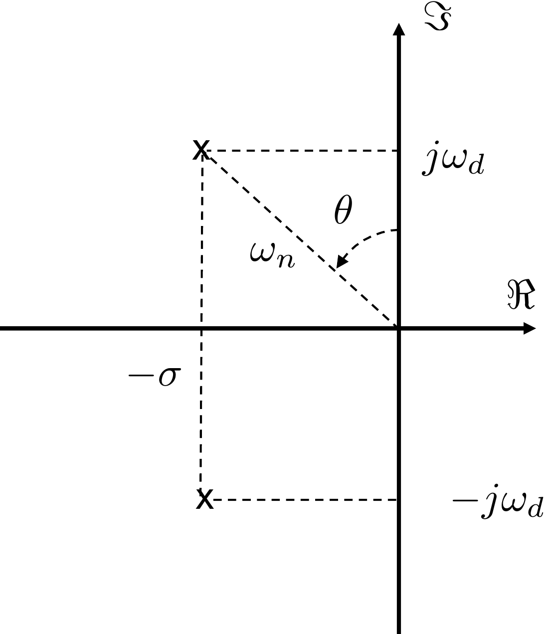
Fig.8.5, where \(\omega_n\) is the distance from the origin
to the poles. When \(\zeta=\frac{1}{\sqrt{2}}\) the angle \(\theta\) equals \(45\) degrees.
Figure 8.5. Complex conjugate poles in the left
half-plane.
In rectangular coordinates, the poles are given by \[\tag{8.3}
p_{1,2} = -\sigma \pm j\omega_d,\] as shown in
Fig.8.5.
Equations 8.2
and 8.3
give \[\begin{aligned}
\sigma &= \zeta \omega_n \\
\omega_d &= \omega_n\sqrt{1-\zeta^2}.
\end{aligned}\] From
Fig.8.5 it is also clear that
\[\sin\theta = \frac{\sigma}{\omega_n} =
\zeta.\] Therefore \[\theta =
\sin^{-1} \zeta.\]
Since the pole locations are at \(-\zeta\omega_n \pm
\omega_n\sqrt{\zeta^2-1}\), the poles are both real if \(\zeta\geq 1\). When \(\zeta=1\) the poles are both located at
\(-\omega_n\). When \(0<\zeta<1\) the poles are imaginary
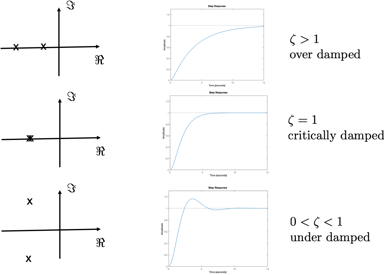
and occur in complex conjugate pairs. As shown in
Fig.8.6, we say that the system
is overdamped when \(\zeta>1\), we say that the system is
critically damped when \(\zeta=1\), and we say that the system is
underdamped when \(0<\zeta<1\).
Figure 8.6. Second-order response as a function of
the damping ratio ζ.
Figure 8.6 (Interactive). Adjust damping ratio zeta to see under-damped,
critically-damped, and over-damped regimes.
The response of \(H(s)\) to a step
of size \(A\) is the inverse Laplace
transform of \[Y(s) =
\frac{A\omega_n^2}{s(s^2+2\zeta\omega_n s + \omega_n^2)},\]
which, as shown in
Appendix 29, when the poles are
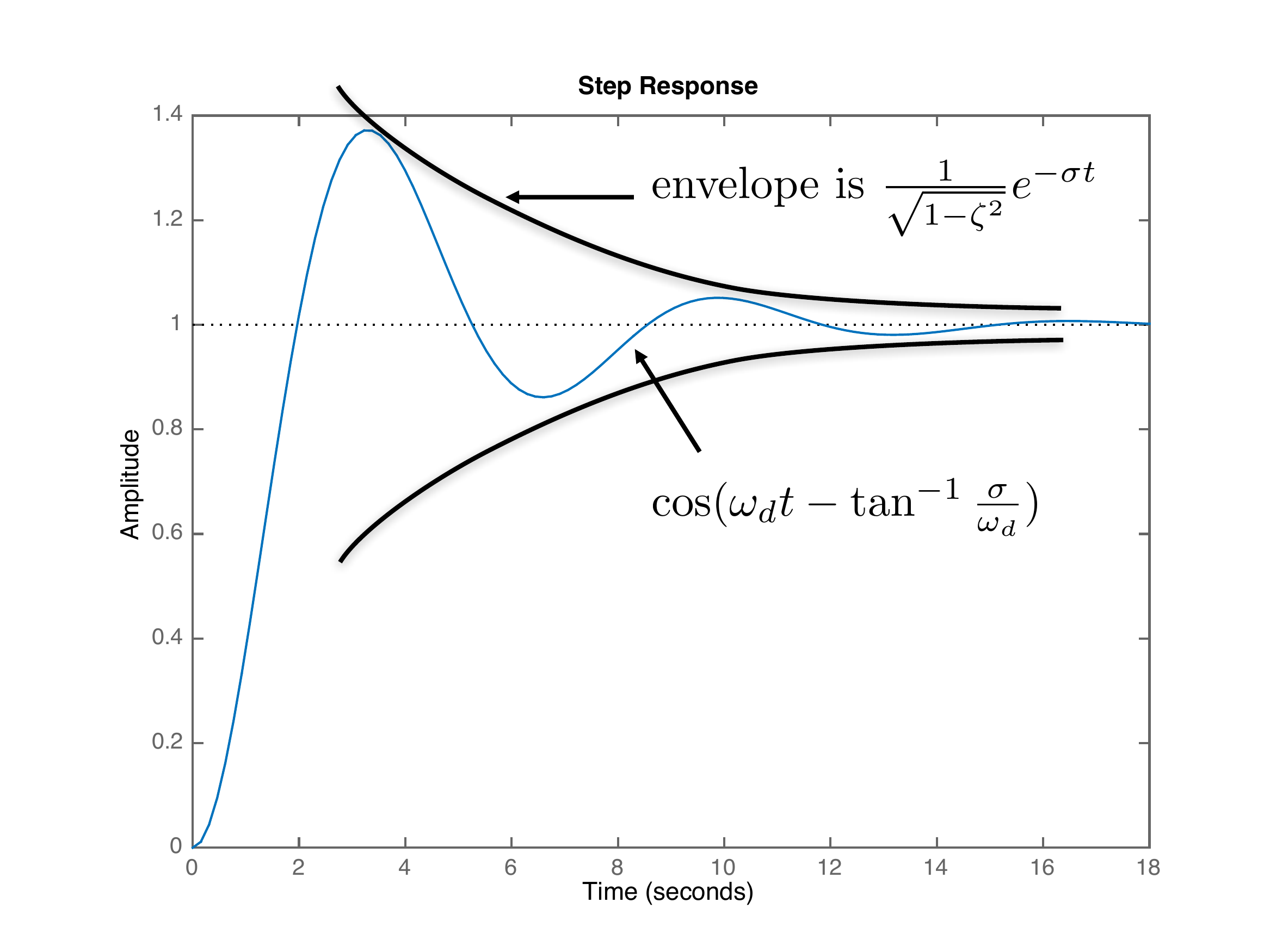
complex results in \[\tag{8.4}
y(t) = A\left[ 1-\frac{1}{\sqrt{1-\zeta^2}}e^{-\sigma
t}\cos\left(\omega_d t -
\tan^{-1}\left(\frac{\sigma}{\omega_d}\right)\right)\right].\] A
plot of this signal is shown in
Fig.8.7.
Figure 8.7. Second-order response. The steady-state
value is A. The response
envelope decays exponentially, and the oscillation frequency and phase
shift are set by the complex pole locations.
The rise time is defined to be the
time that it takes the output to transition from 10% to 90% of its final
value \(A\). A suitable approximation
is that the rise time is one half of the peak time, which is the time
when \(y(t)\) reaches its first peak.
To find the peak time \(t_p\),
differentiate \(y(t)\) in
Equation 8.4 and then
solve for the first instance when the derivative is zero. The result is
\[t_p = \frac{\pi}{\omega_d} =
\frac{\pi}{\omega_n\sqrt{1-\zeta^2}}.\] Therefore, the rise time
is approximately \[t_r \approx \frac{1}{2}t_p
= \frac{1}{2}\frac{\pi}{\omega_n\sqrt{1-\zeta^2}}.\] When \(\zeta=0.707\) we get \[\tag{8.5}
t_r \approx \frac{2.2}{\omega_n}.\]
Specifications for second-order systems are usually given either in
terms of the rise time \(t_r\) and the
damping ratio \(\zeta\), or in terms of
the natural frequency \(\omega_n\) and
the damping ratio \(\zeta\).
8.1.3 Effect of a Zero on the Step
Response
In the previous section, we looked at the step response when there
were two complex poles and no zeros. In this section we will briefly
discuss the effect of zeros on the step response
of the system. This is a topic that
we could treat at a much deeper level.
A transfer function is called rational if it is the ratio of
two polynomials in \(s\). For example,
\[H(s) = \frac{s+1}{s^3+3s^2+s+4}\] is
a rational transfer function, whereas \[H(s)
= \frac{(s+1)e^{-s}}{s^3+3s^2+s+4}\] is not. A rational transfer
function can be written as \[H(s) =
\frac{N(s)}{D(s)},\] where \(N(s)\) is the numerator polynomial and
\(D(s)\) is the denominator polynomial.
The zeros of the transfer function are roots of the equation
\(N(s)=0\), and the poles of the system
are the roots of the equation \(D(s)=0\).
One way to understand the effect of zeros is to consider the effect
that zeros have on the partial fraction expansion of a transfer
function. For a review of partial fraction expansion, see
Appendix 29. First consider a
two-pole system with characteristic equation given by \(\Delta(s) = (s+2)(s+3)\). The transfer
function with DC gain equal to one and without zeros is given by \[H(s) = \frac{6}{(s+2)(s+3)}.\] The
response to a unit step is given by \begin{align}
y(t) &= \mathcal{L}^{-1}\left\{\frac{6}{s(s+2)(s+3)}\right\} \notag
\\
&= \mathcal{L}^{-1}\left\{ \frac{1}{s} + \frac{-3}{s+2} +
\frac{2}{s+3}\right\} \notag \\
&= 1 - 3e^{-2t} + 2e^{-3t}, \quad t\geq 0.
\tag{8.6}
\end{align} Now consider the step response when a zero has
been added at \(z=-2.1\) and the gain
adjusted so that the DC gain is still one, i.e., when \[H(s) =
\frac{\frac{6}{2.1}(s+2.1)}{(s+2)(s+3)}.\] The response to a unit
step is given by \[\begin{aligned}
y(t) &=
\mathcal{L}^{-1}\left\{\frac{\frac{6}{2.1}(s+2.1)}{s(s+2)(s+3)}\right\}
\\
&= \mathcal{L}^{-1}\left\{ \frac{1}{s} + \frac{-0.1429}{s+2} +
\frac{-0.8571}{s+3}\right\}\\
&= 1 - 0.1429e^{-2t} - 0.8571e^{-3t}, \quad t\geq 0.
\end{aligned}\] Note that \(y(t)\) still settles to one, but the
response of the pole at \(-2\) has
almost been removed. If, however, the zero is far away from the poles,
then the effect is much less. Suppose that the zero is at \(z=-60\) and the gain is adjusted so that
the DC gain is still one, i.e., \[H(s) =
\frac{\frac{6}{60}(s+60)}{(s+2)(s+3)}.\] The response to a unit
step is given by \[\begin{aligned}
y(t) &=
\mathcal{L}^{-1}\left\{\frac{\frac{6}{60}(s+60)}{s(s+2)(s+3)}\right\} \\
&= \mathcal{L}^{-1}\left\{ \frac{1}{s} + \frac{-2.9}{s+2} +
\frac{1.9}{s+3}\right\}\\
&= 1 - 2.9e^{-2t} + 1.9e^{-3t}, \quad t\geq 0.
\end{aligned}\] In this case, the response is similar to
Equation 8.6.
Another way to understand the effect of zeros on the system is to
recall that an \(s\) in the numerator
is essentially a differentiator. Therefore \[\begin{aligned}
H(s) &= \frac{\omega_n^2(\tau s+1)}{s^2 + 2\zeta\omega_n s +
\omega_n^2} \\
&= \tau\frac{\omega_n^2 s}{s^2 + 2\zeta\omega_n s + \omega_n^2}
+ \frac{\omega_n^2}{s^2 + 2\zeta\omega_n s + \omega_n^2}.
\end{aligned}\] Therefore, the step response is given by \[\begin{aligned}
y(t) &= \mathcal{L}^{-1}\left\{\tau\frac{\omega_n^2s}{s(s^2 +
2\zeta\omega_n s + \omega_n^2)} + \frac{\omega_n^2}{s(s^2 +
2\zeta\omega_n s + \omega_n^2)}\right\} \\
&= \tau\frac{d}{dt}\mathcal{L}^{-1}\left\{\frac{\omega_n^2}{s(s^2 +
2\zeta\omega_n s + \omega_n^2)}\right\}
%
+ \mathcal{L}^{-1}\left\{\frac{\omega_n^2}{s(s^2 + 2\zeta\omega_n s
+ \omega_n^2)}\right\}.
\end{aligned}\] Therefore, the effect of the zero is to add \(\tau\) times the derivative of the step
response to what the step response would have been without the zero.
Fig.8.8
shows the step response for different values of \(\tau\), illustrating that adding a zero has
a strong effect on the rise time and damping of the response. Note also
that when \(\tau<0\), i.e., when
zeros are in the right half-plane, the system response first goes
negative before going positive. Right-half-plane zeros are often called
nonminimum-phase zeros , and the associated
response is often called a nonminimum-phase response. Physical systems
that have right-half-plane zeros include the inverted pendulum and
aircraft altitude-control systems. For the inverted pendulum, to move
the cart to the right from a stopped position, the cart must first move
left so that the rod leans right before the cart can move to its desired
position. Similarly, an aircraft pitches up to climb. However, when the
aircraft pitches up, it loses speed, which causes it to lose lift and
altitude. As the aircraft loses altitude, it gains speed and produces
the lift necessary to climb.
Figure 8.8.
Interactive step response of a second-order system with a single zero.
Vary tau to see the effect of left-half-plane and right-half-plane zero
behavior.
8.1.4 Successive Loop Closure
The natural frequency \(\omega_n\)
and the damping ratio \(\zeta\) are
only defined for second-order systems, and therefore, the PD design
technique based on \(\omega_n\) and
\(\zeta\) are only valid for
second-order systems. However, these concepts can be extended to
higher-order systems through a technique called successive loop
closure, or inner-loop,
outer-loop design. When we derived the Laplace transform in
Chapter 8, we saw that for
many systems, the transfer functions can be arranged in cascade form as
shown in
Fig.8.9 where the input to the
system is \(u_1\) and the output is
\(y_2\), but where \(y_1\) and \(u_2\) are intermediary values that
represent the natural physical coupling between internal variables. Many
physical systems can be represented by a cascade of systems.
Figure 8.9. Open-loop transfer function modeled as a
cascade of two transfer functions.
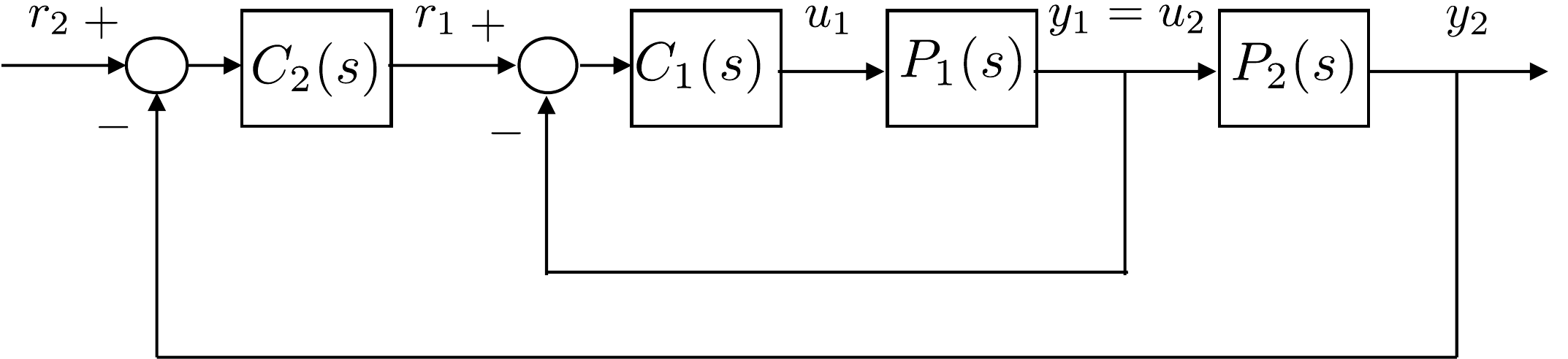
When the system is represented as a cascade, the control strategy can
be designed using successive loop closure. The basic idea is to
close feedback loops in succession around the open-loop plant dynamics
rather than designing a single control system. To illustrate this
approach, consider the open-loop system shown in
Fig.8.9. The open-loop dynamics
are given by the product of two transfer functions in series: \(P(s)=P_1(s)P_2(s)\). We assume that each of
the transfer functions has an output (\(y_1\), \(y_2\)) that can be measured and used for
feedback. Typically, each of the transfer functions, \(P_1(s)\) and \(P_2(s)\), is of relatively low order –
usually first or second-order. In this case, we are interested in
controlling the output \(y_2\). Instead
of closing a single feedback loop around \(y_2\), we will close feedback loops around
\(y_1\) and \(y_2\) in succession as shown in
Fig.8.10.
Figure 8.10. Successive loop closure
design.
We will design the compensators \(C_1(s)\) and \(C_2(s)\) in succession. A necessary
condition in the design process is that the inner loop must be much
faster than each successive loop. As a rule of thumb, if the rise time
of the inner loop is \(t_{r_1}\), the
rise time of the next loop should be 5 to 10 times longer, i.e., \(t_{r_2}> W_1 t_{r_1}\), where \(W_1\) is a design parameter, usually on the
order of \(5-10\). In
part V of this book,
we will talk about the frequency response of the system. At that time,
we will provide a deeper explanation that can be understood in terms of
the bandwidth of each successive loop.
Examining the inner loop shown in
Fig.8.10, the goal is to design a
closed-loop system from \(r_1\) to
\(y_1\) having a rise time of \(t_{r_1}\). If the rise time of the inner
loop is significantly faster than the rise time of the outer loop, and
if the DC gain of the inner loop is
\(k_{DC_1}\), then relative to the
outer loop the inner loop can be effectively modeled as the DC gain.
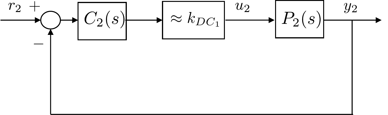
This is depicted schematically in
Fig.8.11. With the inner-loop
transfer function modeled as its DC gain, design of the outer loop is
simplified because it only includes the plant transfer function \(P_2(s)\) and the compensator \(C_2(s)\) and the DC gain \(k_{DC_1}\).
Figure 8.11. Successive loop closure design with inner
loop modeled as a unity gain.
Because both plant models \(P_1(s)\)
and \(P_2(s)\) are first or
second-order, conventional PID compensators can be employed. The
loopshaping techniques discussed in
Part V can also be
used for successive loop closure of higher-order systems.
8.1.5 Input Saturation and Limits
of Performance
A natural question is to ask if the rise time can be made arbitrarily
small. Unfortunately, saturation limits on the actuators place a lower
bound on the achievable rise time. All physical systems have saturation
limits on their actuators. For example, in the robot arm problem, the
torque that can be applied to the arm is limited by the motor that is
used to apply that torque. Force and torque will always be limited by
physical constraints like current limits. Similarly, for an airplane,
the rudder command is limited by how far the rudder can physically move,
which is typically on the order of \(\pm
40\) degrees. A natural way to model input constraints is to add
a saturation block preceding the physical plant.
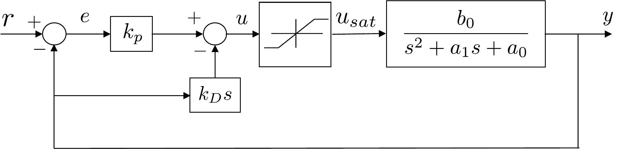
Fig.8.12 shows a saturation
block in conjunction with a PD control scheme.
Figure 8.12. Control system with input saturation. The
input saturation places a lower bound on the achievable rise
time.
Mathematically, the saturation block is given by \[u_{sat} = \begin{cases}
u_{\max}, & \text{~if~} u\geq u_{\max} \\
u, & \text{~if~} -u_{\max} \leq u \leq u_{\max} \\
-u_{\max}, & \text{~otherwise}
\end{cases},\] where the input to the block is \(u\), the output is \(u_{sat}\), and the saturation limit is
\(u_{\max}\). Note that the saturation
block is non-linear. Therefore, one design strategy is to select the
feedback gains so that the system remains linear by keeping the input
out of saturation.
To see how this might be done, consider the second-order system shown
in
Fig.8.12 with proportional
feedback on the output error and derivative feedback on the output. When
the input is not saturated, the closed-loop transfer function is \[Y(s) = \left(\frac{b_0 k_p}{s^2 + (a_1 + b_0
k_D)s + (a_0 + b_0 k_p)}\right) R(s).
\tag{8.7}\] We can see that the closed-loop
poles of the system are defined by the selection of the control gains
\(k_p\) and \(k_D\). Note also that the actuator effort
\(u\) can be expressed as \(u=k_p e - k_D\dot{y}\). When \(\dot{y}\) is zero or small, the size of the
actuator effort \(u\) is primarily
governed by the size of the control error \(e\) and the control gain \(k_p\). If the system is stable, the largest
control effort in response to a step input will occur immediately after
the step when \(\dot{y}=0\). If the
system is to be kept just out of saturation, then immediately after the
step we have \(\left|u\right|=u_\text{max} =
k_p e_\text{max}\). Rearranging this expression, we find that the
proportional control gain can be determined from the maximum anticipated
output error and the saturation limits of the actuator as \[k_p = \pm \frac{u_\text{max}}{e_\text{max}},
\tag{8.8}\] where \(u_{\max}\) is the maximum control effort
the system can provide, \(e_{\max}\) is
the step error that results from a step input of nominal size, and the
sign of \(k_p\) is determined by the
physics of the system.
Suppose that the desired closed-loop characteristic polynomial is
given by \[\Delta_{cl}^d(s) = s^2 +
2\zeta\omega_n s + \omega_n^2,\] then by comparing with the
actual closed-loop characteristic polynomial \[\Delta_{cl}(s) = s^2 + (a_1 + b_0 k_D)s + (a_0 +
b_0 k_p)\] we have that \[\begin{aligned}
\omega_n &= \sqrt{a_0 + b_0 k_p}
\leq \sqrt{a_0 + b_0 \frac{u_\text{max}}{e_\text{max}}},
\end{aligned}\] which is an upper limit on the natural frequency
of the closed-loop system, ensuring that saturation of the actuator is
avoided. The corresponding rise time constraint is \[t_r \geq \frac{2.2}{\omega_n} =
\frac{2.2}{\sqrt{a_0 + b_0 \frac{u_\text{max}}{e_\text{max}}}},\]
which is the smallest possible rise time for an error step of \(e_{\text{max}}\).
If the input has an equilibrium value, then the saturation constraint
used in the above calculation must be modified to account for the
equilibrium. For example, suppose that \(u=u_e+\tilde{u}\) where \(u_e\) is the equilibrium value and \(\tilde{u}\) is the output of the PID
controller. Also suppose that the input saturation constraint is given
by \(u_{\min}\leq u\leq u_{\max}\). The
objective is to find a value for \(\tilde{u}_{\max}\) where \(\left|\tilde{u}\right|\leq
\tilde{u}_{\max}\) guarantees that \(u_{\min}\leq u\leq u_{\max}\). We have that
\[\begin{aligned}
& u_{\min}\leq u \leq u_{\max} \\
\implies & u_{\min} \leq u_e + \tilde{u} \leq u_{\max} \\
\implies & u_{\min}-u_e \leq \tilde{u} \leq u_{\max}-u_e.
\end{aligned}\] The desired value for \(\tilde{u}_{\max}\) is therefore the minimum
(in absolute value) of the right and left-hand sides of this expression.
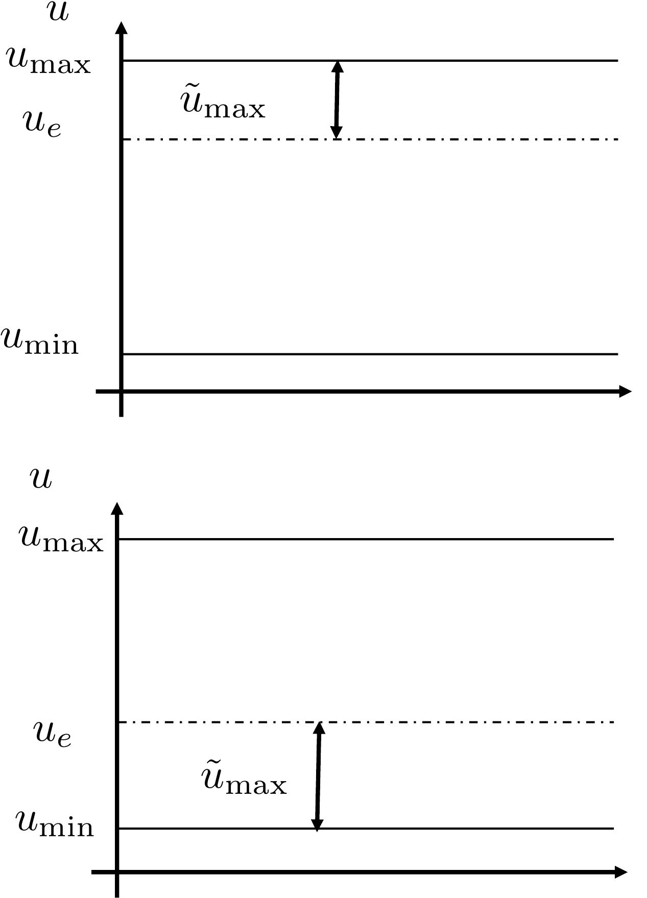
The situation is shown in
Fig.8.13, where it is clear
that the value for \(\tilde{u}_{\max}\)
can be written as \[\tilde{u}_{\max} =
\begin{cases}
\left|u_{\max}-u_e\right|, & \text{~if~} u_e \geq
\frac{u_{\max}+u_{\min}}{2} \\
\left|u_e - u_{\min}\right|, & \text{~if~} u_e \leq
\frac{u_{\max}+u_{\min}}{2}.
\end{cases}\]
Figure 8.13. The saturation constraint for ũ depends on the value of the
equilibrium input ue.
The takeaway from this discussion is that the rise time is limited by
the input saturation constraint and cannot be made arbitrarily small. In
practice, the control parameters are tuned so that the closed-loop
system has the fastest possible rise time without driving the plant
input into saturation.
(a) Suppose that the design requirements are that the rise time is \(t_r \approx 0.8\) seconds, with a damping
ratio of \(\zeta=0.707\). Find the
desired closed-loop characteristic polynomial \(\Delta_{cl}^d(s)\) and the associated pole
locations. Find the proportional and derivative gains \(k_P\) and \(k_D\) to achieve these specifications, and
modify the simulation from
HW 3.1.8 to verify that the step
response satisfies the requirements.
(b) Suppose that the input torque for the robot arm is limited to \(\left|\tau\right|\leq\tau_{\max}=1\) Nm.
Modify the simulation to include a saturation on the torque \(\tau\). Using the rise time \(t_r\) and damping ratio \(\zeta\) as tuning parameters, tune the PD
control law so that the input just saturates when a step of size \(50\) degrees is placed on \(\tilde{r}_{\theta}\).
Design Study A guided exercise
Use rise time and damping ratio
Translate the
time-domain design specifications into a desired second-order
polynomial.
Step 1. Natural frequency rule
Show solution
for Step 1
Answer: Use \(\omega_n\approx 2.2/t_r\).
Step 2. Desired polynomial coefficients
Show solution for Step
2
Answer: The standard form is
\(s^2+2\zeta\omega_n s+\omega_n^2\).
Step 3. Saturation check
Show solution for Step
3
Answer: The gains can satisfy the
linear pole placement equations but still demand torque beyond the
actuator limit.
Pseudocode
The complete solution includes a PD
controller class and a simulation script. Before opening it, outline
each component separately.
These prompts are ungraded. They are
intended to connect the design specifications to the implementation code
in the complete solution.
Complete solution
A rise time of \(t_r\approx 0.8\)
seconds, implies that the natural frequency is \[\omega_n = 2.2/0.8 = 2.75.\] Therefore,
the desired characteristic polynomial is \[\tag{8.9}
\Delta_{cl}^d = s^2 + 2\zeta\omega_n s + \omega_n^2 = s^2 + 3.889 s +
7.5625.\] From HW 3.1.7
the actual closed-loop characteristic polynomial is \[\tag{8.10}
\Delta_{cl}(s) = s^2 + (0.667 + 66.67k_D)s + 66.67k_P.\] Equating
Equations 8.9 and 8.10
and solving for the gains gives \[\begin{aligned}
k_P &= 0.1134 \\
k_D &= 0.0483.
\end{aligned}\]
A Python class that implements a PD controller for the single link
robot arm is shown below.
# 3rd-partyimport numpy as np# local (controlbook)import case_studies.A_arm.params as Pfrom case_studies.common.controller_base import ControllerBaseclass ArmControllerPD(ControllerBase):def__init__(self, use_feedback_linearization: bool=True):# tuning parameters p1 =-3.0 p2 =-4.0# system parameters b0 = P.tf_num[-1] a1, a0 = P.tf_den[-2:]# desired characteristic equation parameters# des_CE: s^2 + alpha1*s + alpha0 = s^2 + (a1 + b0*kd)s + (a0 + b0*kp) des_CE = np.poly([p1, p2]) alpha1, alpha0 = des_CE[-2:]# find gainsself.kp = (alpha0 - a0) / b0self.kd = (alpha1 - a1) / b0print(f"{self.kp =:.2f}, {self.kd =:.3f}")self.tau_eq = P.tau_eqself.use_feedback_linearization = use_feedback_linearizationdef update_with_measurement(self, r, y):raiseNotImplementedError("This controller only uses state feedback.")def update_with_state(self, r, x):# unpack references and states theta_ref = r[0] theta, thetadot = x# theta (modified) PD error = theta_ref - theta tau_tilde =self.kp * error -self.kd * thetadotifself.use_feedback_linearization: tau_fl = P.m * P.g * P.ell /2* np.cos(theta) tau = tau_tilde + tau_flelse: # use equilibrium (Jacobian linearization)# NOTE: likely not work well (or at all) for large angles tau = tau_tilde +self.tau_eq u = np.array([tau])return u
Code that computes the control gains is given below.
(a) Using the principle of successive loop closure, draw a block diagram
that uses PD control for both inner loop control and outer loop control.
The input to the outer loop controller is the desired cart position
\(r_z\) and the output of the
controller is the desired pendulum angle \(r_{\theta}\). The input to the inner loop
controller is the desired pendulum angle \(r_{\theta}\) and the output is the force
\(F\) on the cart.
(b) Focusing on the inner loop, find the PD gains \(k_{P_\theta}\) and \(k_{D_\theta}\) so that the rise time of the
inner loop is \(t_{r_\theta}=0.5\) seconds, and the damping
ratio is \(\zeta_{\theta}=0.707\).
(c) Find the DC gain \(k_{DC_\theta}\) of
the inner loop.
(d) Replace the inner loop by its DC gain and consider the outer loop. Add a
low-pass filter that cancels the left-half-plane zero, and then design a
PD control strategy to stabilize the position of the cart.
(e) Implement the control design to control on the inverted pendulum. Modify
the simulation to include saturation on the force \(F\) to limit the size of the input force on
the cart to \(F_{\max}=5\) N. Give the
pendulum angle an initial condition of 10 deg and simulate the response
of the system for 10 seconds to verify that the cart is able to balance
the pendulum. You may also tune rise times or damping to improve
performance.
Design
Study B guided exercise
Organize the successive-loop
pendulum controller
Separate the inner angle loop from the
outer cart-position loop.
The inner loop stabilizes pendulum angle
before the outer loop commands cart position.
Step 1. Loop signal order
Show solution for Step
1
Answer: The outer position
command produces an angle command, which the inner loop converts to
force.
Step 2.
Inner-loop design target
Show
solution for Step 2
Answer: The
inner loop controls theta with a 0.5 second rise-time
target.
Step 3.
Outer-loop design feature
Show
solution for Step 3
Answer: A
low-pass filter is added in the outer loop to cancel the left-half-plane
zero.
Pseudocode
The complete solution includes a nested PD
controller class and a zero-canceling filter class. Before opening it,
outline each component separately.
These prompts are
ungraded. They are intended to connect the derivation to the
implementation code in the complete solution.
Complete solution
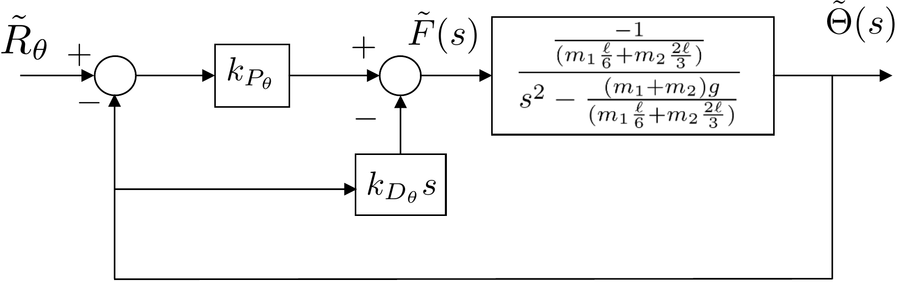
The block diagram for the inner loop is shown in
Fig.8.14.
Figure 8.14. Block diagram for inner loop of inverted
pendulum control
The closed-loop transfer function from \(\tilde{R}_{\Theta}\) to \(\tilde{\Theta}\) is given by \[\tilde{\Theta}(s) =
\frac{-\frac{k_{P_\theta}}{m_1 \frac{\ell}{6} +m_2\frac{2\ell}{3}}}{s^2
- \frac{k_{D_\theta}}{m_1 \frac{\ell}{6}
+m_2\frac{2\ell}{3}}s-\left(\frac{(m_1+m_2)g}{m_1 \frac{\ell}{6}
+m_2\frac{2\ell}{3}}+\frac{k_{P_\theta}}{m_1 \frac{\ell}{6}
+m_2\frac{2\ell}{3}}\right)} \tilde{R}_{\Theta}(s).\] Therefore,
the closed-loop characteristic equation is \[\Delta_{cl}(s) =s^2 - \frac{k_{D_\theta}}{m_1
\frac{\ell}{6} +m_2\frac{2\ell}{3}}s-\left(\frac{(m_1+m_2)g}{m_1
\frac{\ell}{6} +m_2\frac{2\ell}{3}}+\frac{k_{P_\theta}}{m_1
\frac{\ell}{6} +m_2\frac{2\ell}{3}}\right)\] The desired
closed-loop characteristic equation is \[\Delta_{cl}^d(s) = s^2 +
2\zeta_{\theta}\omega_{n_\theta} s + \omega_{n_\theta}^2,\] where
\[\begin{aligned}
\omega_{n_\theta} &= \frac{2.2}{t_{r_\theta}} = 4.4 \\
\zeta_{\theta} &= 0.707.
\end{aligned}\] Therefore \[\begin{aligned}
k_{P_\theta} &= -(m_1+m_2)g - \left(m_1 \frac{\ell}{6}
+m_2\frac{2\ell}{3}\right)\omega_{n_\theta}^2 = -26.0 \\
k_{D_\theta} &= -2\zeta_{\theta}\omega_{n_\theta}\left (m_1
\frac{\ell}{6} +m_2\frac{2\ell}{3}\right) = -4.41.
\end{aligned}\] The DC gain of the inner loop is given by \[k_{DC_{\theta}} =
\frac{k_{P_\theta}}{(m_1+m_2)g+k_{P_\theta}} = 1.89.\]
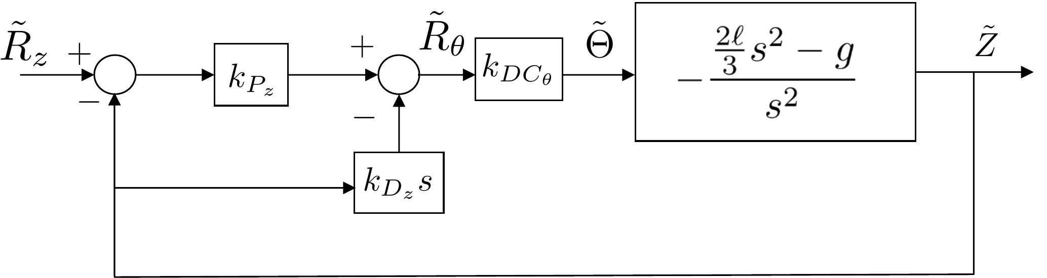
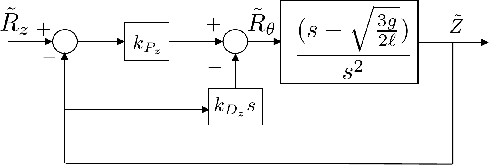
Replacing the inner loop by its DC gain, the block diagram for the
outer loop is shown in Fig.8.15.
Figure 8.15. Block diagram for outer loop of inverted
pendulum control.
The closed-loop transfer function from \(\tilde{R}_z\) to \(\tilde{Z}\) is given by \[\tilde{Z}(s) =
\frac{\frac{k_{P_z}}{k_{D_z}}(s^2-\frac{3g}{2\ell})}{s^3 + s^2 (\frac{
k_{P_z}}{k_{D_z}}-\frac{3}{2 k_{DC_\theta} k_{D_z} \ell} ) - s \frac{3
g}{2 \ell} - \frac{3 k_{P_z} g}{2 k_{D_z} \ell}} \tilde{R}_z.\]
Note that the DC gain for the outer loop is equal to one. The
closed-loop characteristic equation is \[\Delta_{cl}(s) = s^3 + s^2 (\frac{
k_{P_z}}{k_{D_z}}-\frac{3}{2 k_{DC_\theta} k_{D_z} \ell}) - s \frac{3
g}{2 \ell} - \frac{3 k_{P_z} g}{2 k_{D_z} \ell}.\] Since the
desired characteristic equation is \[\tag{8.11}
\Delta_{cl}^d(s) = s^2 + 2\zeta_z\omega_{n_z}s +
\omega_{n_z}^2,\] it is not possible to pick PD gain values that
will create a match between the actual characteristic equation and the
desired characteristic equation.
To resolve this problem, note that the transfer function of the outer
loop can be written as \[H(s) =
\frac{-\frac{2\ell}{3}s^2 + g}{s^2}
= \frac{-\frac{2\ell}{3}(s +
\sqrt{\frac{3g}{2\ell}})(s-\sqrt{\frac{3g}{2l}})}{s^2},\] where
we see that the system has two zeros, one in the right half-plane and
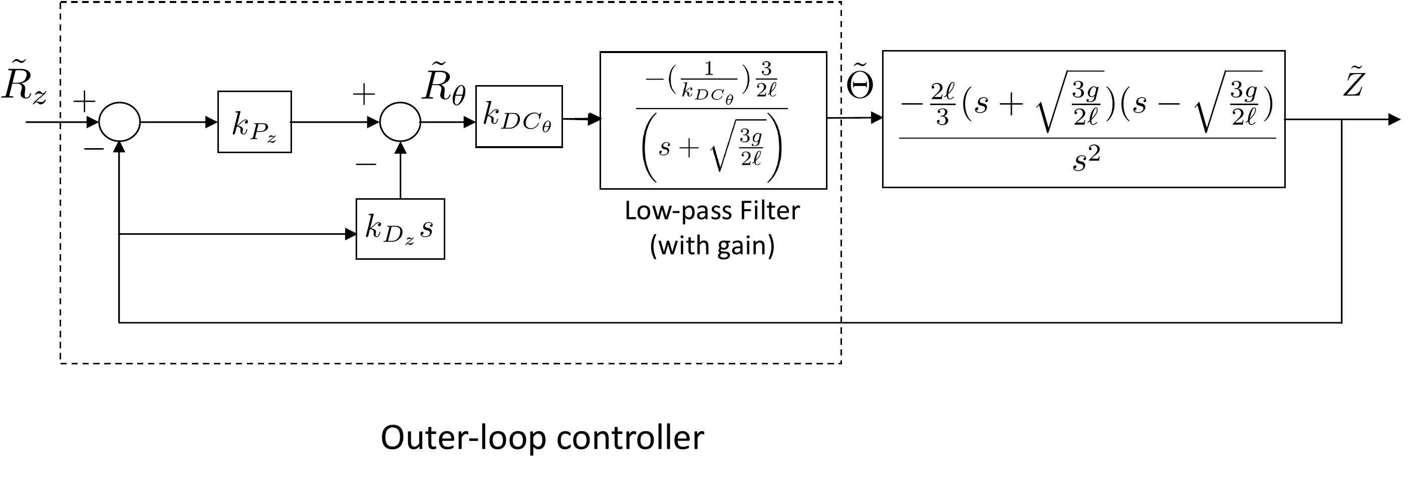
one in the left half-plane. The strategy for making the numerator
polynomial have degree one is to add a low-pass filter after the PD
controller that attempts to cancel the left-half-plane zero, as shown in
Figure 8.16. An important
part of this filter is also including an additional gain to cancel the
effect of \(K_{DC_\theta}\), which is
not one.
Figure 8.16. Block diagram for outer loop of inverted
pendulum control, with low-pass filter to cancel the LHP
zero.
After accounting for the cancellations introduced by the low-pass
filter, the equivalent closed-loop system is shown in Figure 8.17.
Figure 8.17. Block diagram for the equivalent outer
loop of inverted pendulum control with low-pass filter.
In this case, the closed-loop characteristic equation from \(\tilde{R}_z\) to \(\tilde{Z}\) is given by \[\tilde{Z}(s) = \left(
\frac{\left(\frac{k_{P_z}}{1+k_{D_z}}\right)
(s-\sqrt{\frac{3g}{2\ell}})}
{s^2 + \left(\frac{k_{P_z} -
k_{D_z}\sqrt{\frac{3g}{2\ell}}}{1+k_{D_z}}\right)s -
\frac{k_{P_z}\sqrt{\frac{3g}{2\ell}}}{1+k_{D_z}}}
\right) \tilde{R}_z.\] Setting the closed-loop
characteristic equation equal to the desired closed-loop characteristic
equation in Equation 8.11
gives \[\begin{aligned}
- \sqrt{\frac{3g}{2\ell}} \frac{k_{P_z}}{1+k_{D_z}} &=
\omega_{n_z}^2 \\
\frac{k_{P_z}}{1+k_{D_z}} -
\sqrt{\frac{3g}{2\ell}}\frac{k_{D_z}}{1+k_{D_z}} &= 2\zeta_z
\omega_{n_z},
\end{aligned}\] which implies that \[\begin{aligned}
\frac{k_{P_z}}{1+k_{D_z}} &= - \sqrt{\frac{2\ell}{3g}}
\omega_{n_z}^2 \stackrel{\triangle}{=}a \\
\frac{k_{D_z}}{1+k_{D_z}} &= \sqrt{\frac{2\ell}{3g}}
\left[\frac{k_{P_z}}{1+k_{D_z}} - 2\zeta_z \omega_{n_z} \right] \\
&= \sqrt{\frac{2\ell}{3g}} \left[-
\sqrt{\frac{2\ell}{3g}} \omega_{n_z}^2 - 2\zeta_z \omega_{n_z}
\right] \stackrel{\triangle}{=}b.
\end{aligned}\] Solving for the gains in terms of \(a\) and \(b\) gives \[\begin{aligned}
k_{D_z} &= \frac{b}{1-b} \\
k_{P_z} &= \frac{a}{1-b}.
\end{aligned}\]
A Python class that implements a PD controller for the inverted
pendulum is shown below.
# 3rd-partyimport numpy as np# local (controlbook)# TODO: decide whether to use global vs relative imports for public case studies# (it might depend on what you want to show up in the book)import case_studies.B_pendulum.params as Pfrom case_studies.common.controller_base import ControllerBase# from . import params as Pclass CartPendulumControllerPD(ControllerBase):def__init__(self):# tuning parameters tr_theta =0.5# original tr_theta =0.15# tuned to saturate for single time step zeta_theta =0.707 M =10# time separation factor between inner and outer loop tr_z = tr_theta * M zeta_z =0.707# system parameters a1_inner, a0_inner = P.tf_inner_den[-2:] b0_inner = P.tf_inner_num[-1] b2_outer, _, b0_outer = P.tf_outer_num# Inner loop wn_theta =2.2/ tr_theta alpha0_inner = wn_theta**2 alpha1_inner =2* zeta_theta * wn_thetaself.kp_theta = (alpha0_inner - a0_inner) / b0_innerself.kd_theta = (alpha1_inner - a1_inner) / b0_innerprint(f"Inner loop (theta): {self.kp_theta =:.3f}, {self.kd_theta =:.3f}")# DC gain of inner loop DC_gain = (b0_inner *self.kp_theta) / (a0_inner + b0_inner *self.kp_theta)print(f"{DC_gain =:.3f}")# Outer loop wn_z =2.2/ tr_z zero_LHP =-np.sqrt(b0_outer /-b2_outer) a = wn_z**2/ zero_LHP # eq 8.12 from controlbook b = (a -2* zeta_z * wn_z) /-zero_LHP # eq 8.13 from controlbookself.kd_z = b / (1- b)self.kp_z = a * (1+self.kd_z)print(f"Outer loop (z): {self.kp_z =:.3f}, {self.kd_z =:.3f}")self.filter= ZeroCancelingFilter(zero_LHP, DC_gain)def update_with_measurement(self, r, y):raiseNotImplementedError("This controller only uses state feedback.")def update_with_state(self, r, x): z_ref = r[0] z, theta, zdot, thetadot = x# outer loop control error_z = z_ref - z theta_ref_pre =self.kp_z * error_z -self.kd_z * zdot# low-pass filter the reference angle to cancel the zero and DC gain theta_ref =self.filter.update(theta_ref_pre) r[1] = theta_ref # if you want to visualize the "reference" angle# inner loop control error_theta = theta_ref - theta F =self.kp_theta * error_theta -self.kd_theta * thetadot u_unsat = np.array([F]) u =self.saturate(u_unsat, u_max=P.force_max)return uclass ZeroCancelingFilter:def__init__(self, zero_LHP, DC_gain):# TODO: book uses b for numerator coeffcients and a for denominator# coefficients for all of the system transfer functions, so why does it# switch here? (I switched them so b is on top...is that OK?)# system parameters sys_b2 = P.tf_outer_num[0]# low-pass filter parametersself.b0 =1/ (sys_b2 * DC_gain)self.a0 =-zero_LHPself.state =0.0def update(self, input_):# Euler (RK1) integration state_dot =-self.a0 *self.state +self.b0 * input_self.state =self.state + state_dot * P.tsreturnself.state
Complete simulation code for MATLAB, Python, and Simulink can be
downloaded at http://controlbook.byu.edu.
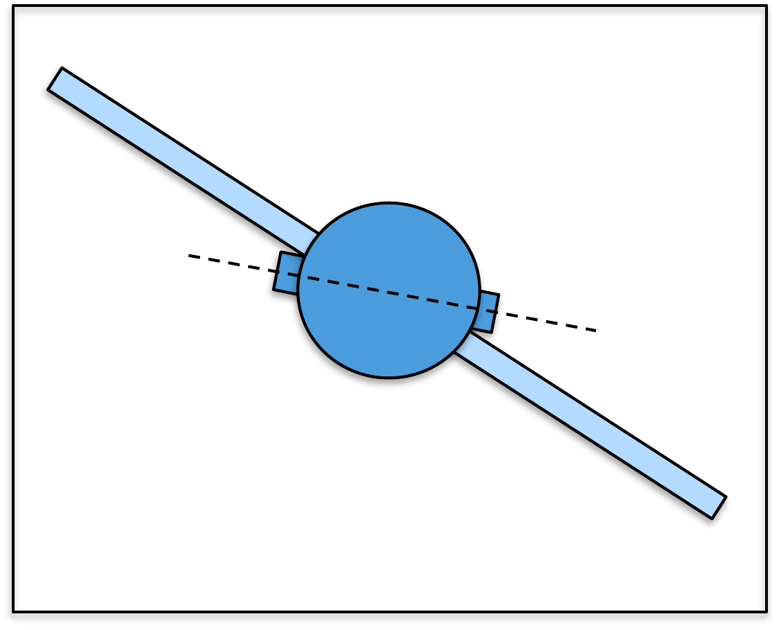
(a) For the simple satellite system, using the principle of successive loop
closure, draw a block diagram that uses PD control for the inner and the
outer loop control. The input to the outer loop controller is the
desired angle of the solar panel \(r_{\phi}\) and the output is the desired
angle of the satellite \(r_{\theta}\).
The input to the inner loop controller is \(r_{\theta}\) and the output is the torque
on the satellite \(\tau\).
(b) Focusing on the inner loop, find the PD gains \(k_{P_\theta}\) and \(k_{D_\theta}\) so that the rise time of the
inner loop is \(t_{r_\theta}=1\) second, and the damping
ratio is \(\zeta_{\theta}=0.9\).
(c) Find the DC gain \(k_{DC_\theta}\) of
the inner loop.
(d) Replacing the inner loop by its DC gain, find the PD gains \(k_{P_\phi}\) and \(k_{D_\phi}\) so that the rise time of the
outer loop is \(t_{r_\phi}= 10
t_{r_\theta}\) with damping ratio \(\zeta_{\phi}=0.9\).
(e) Implement the successive loop closure design for the satellite system in
simulation where the commanded solar panel angle is given by a square
wave with magnitude \(15\) degrees and
frequency \(0.015\) Hz.
(f) Suppose that the size of the input torque on the satellite is limited to
\(\tau_{\max}=5\) Nm. Modify the
simulation to include saturation on the torque \(\tau\). Use rise time as a tuning parameter
and tune the PD control law to get the fastest possible response without
input saturation when a step of size \(30\) degrees is placed on \(r_\phi\).
Design Study C guided exercise
Plan the satellite successive-loop controller
Use the
body loop as the fast inner loop and the flexible-panel loop as the
slower outer loop.
Step 1. Signal
architecture
Show solution for Step
1
Answer: The inner loop controls
\(\theta\) using \(\tau\); the outer loop controls \(\phi\) by commanding \(r_\theta\).
Step 2.
Inner-loop design target
Show solution for
Step 2
Answer: The inner-loop
target is \(t_{r_\theta}=1\) s and
\(\zeta_\theta=0.9\), giving \(k_{DC_\theta}=1\) in the approximation
used here.
Step 3. Outer-loop
separation
Show solution for Step
3
Answer: The outer rise time is
chosen as \(t_{r_\phi}=10t_{r_\theta}\). Faster tuning risks
torque saturation and flexible-panel oscillation.
Pseudocode
Before opening the implementation code,
outline the nested PD controller and saturation check.
Complete solution
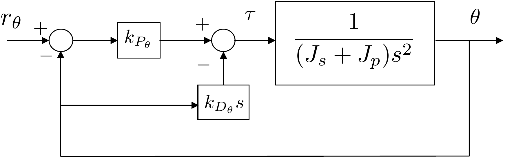
The block diagram for the inner loop is shown in
Fig.8.18.
Figure 8.18. Block diagram for inner loop of satellite
control
The closed-loop transfer function from \(R_{\theta}\) to \(\Theta\) is given by \[%
\Theta(s) = \frac{\frac{k_{P_\theta}}{J_s + J_p}}{s^2
+\left(\frac{k_{D_\theta}}{J_s +
J_p}\right)s+\left(\frac{k_{P_\theta}}{J_s + J_p}\right)}
R_{\theta}(s).\] Therefore, the closed-loop characteristic
equation is \[%
\Delta_{cl}(s) = s^2 +\left(\frac{k_{D_\theta}}{J_s +
J_p}\right)s+\left(\frac{k_{P_\theta}}{J_s + J_p}\right).\] The
desired closed-loop characteristic equation is \[\Delta_{cl}^d(s) = s^2 +
2\zeta_{\theta}\omega_{n_\theta} s + \omega_{n_\theta}^2,\]
where
\[\begin{aligned}
\omega_{n_\theta} &=
\frac{1}{2}\frac{\pi}{t_{r_\theta}\sqrt{1-\zeta_{\theta}^2}} \\
\zeta_{\theta} &= 0.9.
\end{aligned}\] Therefore \[\begin{aligned}
%
k_{P_\theta} &= \omega_{n_\theta}^2(J_s + J_p) = 77.9 \\
%
k_{D_\theta} &= 2\zeta_{\theta}\omega_{n_\theta}(J_s + J_p) = 38.9.
\end{aligned}\] The DC gain of the inner loop is given by \[%
k_{DC_{\theta}} = 1.\]
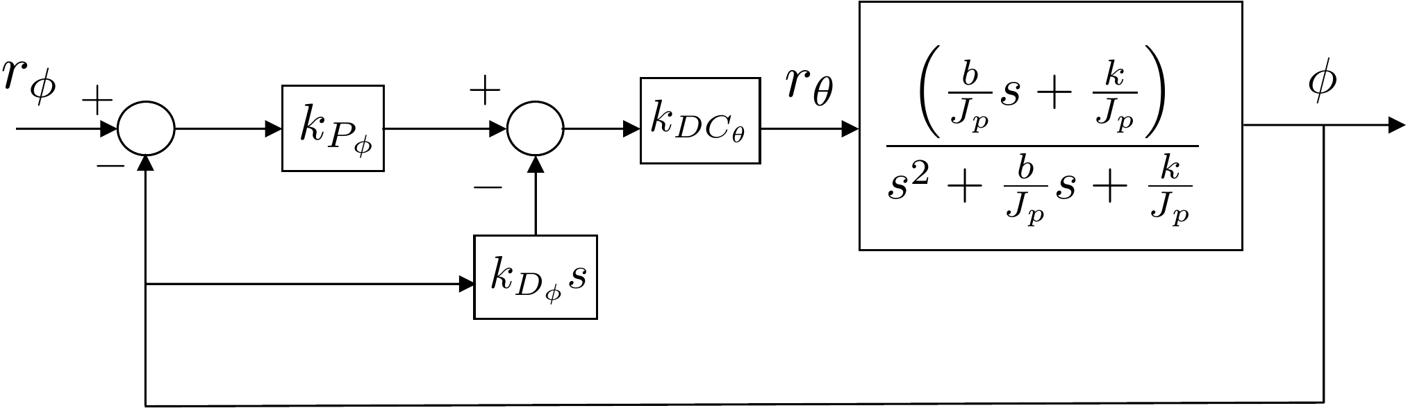
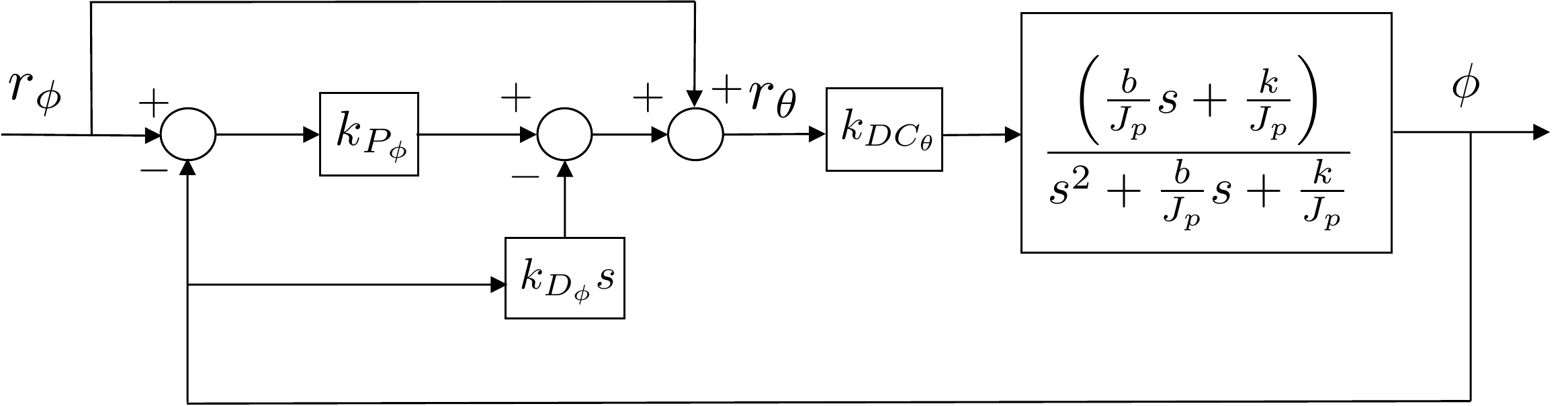
Replacing the inner loop by its DC gain, the block diagram for the
outer loop is shown in Fig.8.19.
Figure 8.19. Block diagram for outer loop of satellite
attitude control
To find the closed-loop transfer function from \(r_{\phi}\) to \(\phi\), follow the loop backwards from
\(\phi\) to obtain \[\Phi(s) =
\left(\frac{\frac{b}{J_p}s+\frac{k}{J_p}}{s^2+\frac{b}{J_p}s+\frac{k}{J_p}}\right)\left[k_{DC_\theta}k_{P_\phi}(\Phi_r-\Phi)-k_{DC_\theta}k_{D_\phi}s\Phi\right].\]
After some manipulation we get \[\begin{gathered}
\big[(J_p+bk_{DC_\theta}k_{D_\phi})s^2 +
(b+bk_{DC_\theta}k_{P_\phi}+kk_{DC_\theta}k_{D_\phi})s
+ (k+kk_{DC_\theta}k_{P_\phi})\big]\Phi \\ =
\left[bk_{DC_\theta}k_{P_\phi}s+kk_{DC_\theta}k_{P_\phi}\right]\Phi_r,
\end{gathered}\] which results in the monic transfer function
\[\Phi(s)=\frac{\left(\frac{bk_{DC_\theta}k_{P_\phi}}{J_p+bk_{DC_\theta}k_{D_\phi}}\right)s+\left(\frac{kk_{DC_\theta}k_{P_\phi}}{J_p+bk_{DC_\theta}k_{D_\phi}}\right)}{s^2
+
\left(\frac{b+bk_{DC_\theta}k_{P_\phi}+kk_{DC_\theta}k_{D_\phi}}{J_p+bk_{DC_\theta}k_{D_\phi}}\right)s
+
\left(\frac{k+kk_{DC_\theta}k_{P_\phi}}{J_p+bk_{DC_\theta}k_{D_\phi}}\right)}
\Phi_r.\] The desired closed-loop characteristic equation for the
outer loop is \[\Delta_{cl}^d(s) = s^2 +
2\zeta_{\phi}\omega_{n_\phi} s + \omega_{n_\phi}^2,\] where \[\begin{aligned}
t_{r_\phi} &= 10~t_{r_\theta} = 10 \\
\omega_{n_\phi} &=
\frac{1}{2}\frac{\pi}{t_{r_\phi}\sqrt{1-\zeta_{\phi}^2}} \\
\zeta_{\phi} &= 0.9.
\end{aligned}\] Therefore, the gains \(k_{P_\phi}\) and \(k_{P_\phi}\) satisfy \[\begin{aligned}
\frac{k+kk_{DC_\theta}k_{P_\phi}}{J_p+bk_{DC_\theta}k_{D_\phi}} &=
\omega_{n_\phi}^2 \\
\frac{b+bk_{DC_\theta}k_{P_\phi}+kk_{DC_\theta}k_{D_\phi}}{J_p+bk_{DC_\theta}k_{D_\phi}}
&= 2\zeta_{\phi}\omega_{n_\phi}.
\end{aligned}\] Expressing these equations in matrix form gives
\[\begin{pmatrix} kk_{DC_\theta} &
-bk_{DC_\theta}\omega_{n_\phi}^2 \\ bk_{DC_\theta} &
kk_{DC_\theta}-2bk_{DC_\theta}\zeta_\phi\omega_{n_\phi}
\end{pmatrix}\begin{pmatrix}k_{P_\phi}\\k_{D_\phi}\end{pmatrix} =
\begin{pmatrix} -k + J_p\omega_{n_\phi}^2 \\ -b +
2J_p\zeta_\phi\omega_{n_\phi} \end{pmatrix},\] implying that
\[\begin{aligned}
%
\begin{pmatrix}k_{P_\phi}\\k_{D_\phi}\end{pmatrix} &=
\begin{pmatrix} kk_{DC_\theta} & -bk_{DC_\theta}\omega_{n_\phi}^2 \\
bk_{DC_\theta} &
kk_{DC_\theta}-2bk_{DC_\theta}\zeta_\phi\omega_{n_\phi}
\end{pmatrix}^{-1}
\begin{pmatrix} -k + J_p\omega_{n_\phi}^2 \\ -b +
2J_p\zeta_\phi\omega_{n_\phi} \end{pmatrix} \\
&= \begin{pmatrix} 0.834 \\ 8.253 \end{pmatrix}
\end{aligned}\]
The DC gain of the outer loop is given by \[%
k_{DC_{\phi}} =
\frac{kk_{DC_\theta}k_{P_\phi}}{k+kk_{DC_\theta}k_{P_\phi}} =
0.455.\] Note that the DC gain of the outer loop is not equal to
one, so there will be significant steady-state error. To remedy this, a
feedforward term can be used to ensure that \(\theta\) and \(\phi\) are made to be equal in steady
state, resulting in an overall DC gain of one. This configuration is
depicted in Fig.8.20.
Feedforward control will be discussed in a later chapter.
Figure 8.20. Block diagram for outer loop of satellite
attitude control with a feedforward term.
A Python class that implements a PD controller using state feedback
is shown below.
# 3rd-partyimport numpy as np# local (controlbook)import case_studies.C_satellite.params as Pfrom case_studies.common.controller_base import ControllerBaseclass SatelliteControllerPD(ControllerBase):def__init__(self):# tuning parameters tr_theta =1.5# original already saturated, so increased rise time. zeta_theta =0.9 M =10# time separation factor between inner and outer loop tr_phi = tr_theta * M zeta_phi =0.9# system parameters a1_inner, a0_inner = P.tf_inner_den[-2:] b0_inner = P.tf_inner_num[-1]# Inner loop wn_theta =0.5* np.pi / (tr_theta * np.sqrt(1- zeta_theta**2)) alpha0_inner = wn_theta**2 alpha1_inner =2* zeta_theta * wn_thetaself.kp_theta = (alpha0_inner - a0_inner) / b0_innerself.kd_theta = (alpha1_inner - a1_inner) / b0_innerprint(f"Inner loop (theta): kp = {self.kp_theta:.3f}, kd = {self.kd_theta:.3f}")# DC gain of inner loop DC_theta = (b0_inner *self.kp_theta) / (a0_inner + b0_inner *self.kp_theta)print(f"{DC_theta =}") # a0 is 0, so DC_gain is 1# Outer loop wn_phi =0.5* np.pi / (tr_phi * np.sqrt(1- zeta_phi**2)) AA = DC_theta * np.array( [ [P.k, -P.b * wn_phi**2], [P.b, P.k - P.b *2* zeta_phi * wn_phi], ] ) bb = np.array([-P.k + P.Jp * wn_phi**2, -P.b + P.Jp *2* zeta_phi * wn_phi])self.kp_phi, self.kd_phi = np.linalg.solve(AA, bb)print(f"Outer loop (phi): kp = {self.kp_phi:.3f}, kd = {self.kd_phi:.3f}")# DC gain of outer loop DC_phi = P.k * DC_theta *self.kp_phi / (P.k + P.k * DC_theta *self.kp_phi)print(f"{DC_phi =:.3f}")self.tau_eq = P.u_eq[0]def update_with_measurement(self, r, y):raiseNotImplementedError("This controller only uses state feedback.")def update_with_state(self, r, x):# unpack references and states phi_ref = r[1] theta, phi, thetadot, phidot = x# outer loop (modified) PD error_phi = phi_ref - phi theta_ref_tilde =self.kp_phi * error_phi -self.kd_phi * phidot theta_ref_ff = phi_ref # feedforward term because outer loop DC gain isn't 1 theta_ref = theta_ref_tilde + theta_ref_ff r[0] = theta_ref # if you want to visualize the "reference" angle# inner loop (modified) PD error_theta = theta_ref - theta tau_tilde =self.kp_theta * error_theta -self.kd_theta * thetadot tau = tau_tilde +self.tau_eq u_unsat = np.array([tau]) u =self.saturate(u_unsat, u_max=P.torque_max)return u
Complete simulation code for MATLAB, Python, and Simulink can be
downloaded at http://controlbook.byu.edu.
8.5 Coding Lab: PD Controller
Implementation
Figure 8.21. Block-diagram setup for the Chapter 8 coding lab on
second-order closed-loop control.
Plant
model used in this lab:
ÿ +
2ζωnẏ +
ωn2y =
ωn2u
Section 8.6 coding lab objective: complete the
controller template and use the targeted checks to evaluate
step-response performance for the second-order system.
Evaluation criteria: rise time ≤ 1.2 s,
overshoot ≤ 20 percent, and steady-state error ≤ 0.03.
Use the code editor to complete the controller class.