F Design Study: Planar VTOL
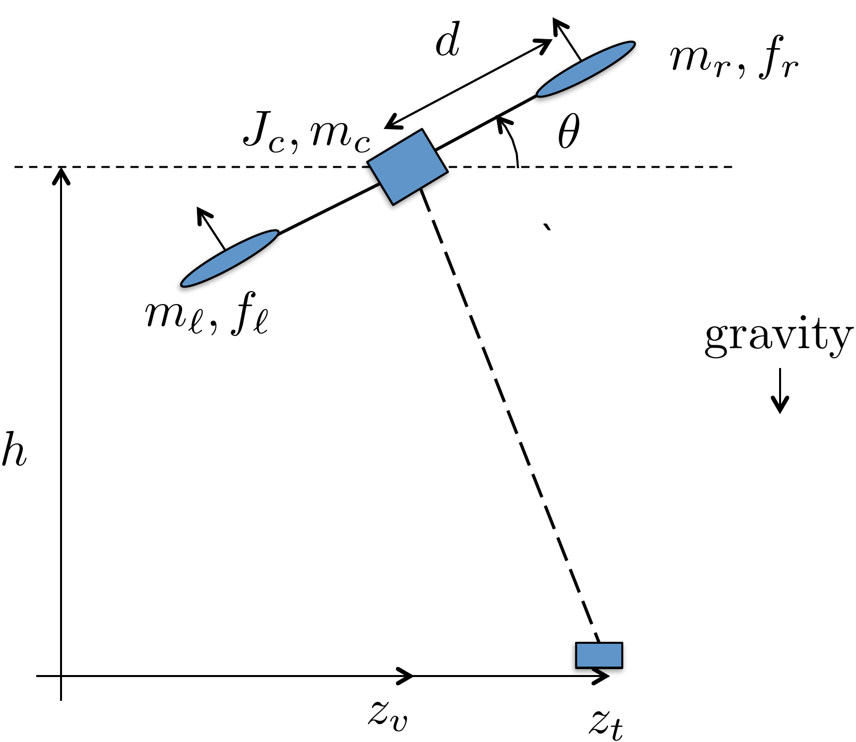
In this design study we explore the control design for a simplified planar version of a quadrotor following a ground target. In particular, we constrain the dynamics to a two-dimensional plane. In Cartesian space, the position of the VTOL can be defined by a variable describing the vertical position, one describing the horizontal position, and one angular variable describing the orientation, as shown in Fig. 21.1. The planar vertical takeoff and landing (VTOL) system consists of a center pod of mass \(m_c\) and inertia \(J_c\), a right motor/rotor that is modeled as a point mass \(m_r\) that exerts a force \(f_r\) at a distance \(d\) from the center of mass, and a left motor/rotor that is modeled as a point mass \(m_\ell\) that exerts a force \(f_\ell\) at a distance \(-d\) from the center of mass. The position of the center of mass of the planar VTOL system is given by horizontal position \(z_v\) and altitude \(h\). The airflow through the rotor creates a change in the direction of flow of air and causes what is called “momentum drag.” Momentum drag can be modeled as a viscous drag force that is proportional to the horizontal velocity \(\dot{z}_v\). In other words, the drag force is \(F_{\text{drag}}=-\mu \dot{z}_v\). The target on the ground will be modeled as an object with position \(z_t\) and altitude \(h=0\). We will not explicitly model the dynamics of the target.
Use the following physical parameters: \(m_c=1\) kg, \(J_c=0.0042\) kg m\(^2\), \(m_r=0.25\) kg, \(m_\ell=0.25\) kg, \(d=0.3\) m, \(\mu = 0.1\) kg/s, \(g=9.81\) m/s\(^2\).
F.2 Kinetic energy.
F.3 Equations of Motion.
F.4 Linearize equations of motion.
F.5 Transfer function model.
F.6 State-space model.
F.7 Pole Placement using PD.
F.8 Successive loop closure.
F.9 Integrators and system type.
F.P.6 Root locus.
F.10 Digital PID.
F.11 Full state feedback.
F.12 Full state with integrator.
F.13 Observer based control.
F.14 Disturbance observer.
F.15 Frequency Response.
F.16 Loop gain.
F.17 Stability margins.
F.18 Loopshaping design.
 Homework F.2
(a) Using the configuration variables \(z_v\), \(h\), and \(\theta\), write an expression for the kinetic energy of the system.
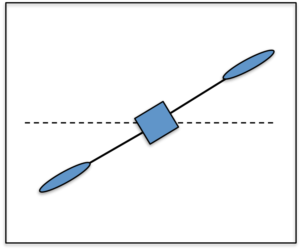
(b) Create an animation of the planar VTOL system. The inputs to the animation should be \(z_v\), \(z_t\), \(h\), and \(\theta\). Turn in a screen capture of the animation.
Homework F.3
(a) Find the potential energy for the system.
(b) Define the generalized coordinates and damping forces.
(c) Find the generalized forces. Note that the right and left forces are more easily modeled as a total force on the center of mass, and a torque about the center of mass.
(d) Derive the equations of motion for the planar VTOL system using the Euler-Lagrange equations.
(e) Referring to Appendices 25, 26, and 27, write a class or s-function that implements the equations of motion. Simulate the system using variable force inputs \(f_r\) and \(f_\ell\). The output should connect to the animation function developed in Homework F.2. Do not be surprised if the system does not behave well (i.e., if the VTOL system seems to crash or go off to infinity). We are simulating an open-loop system with no control to stabilize its behavior.
Homework F.4
Since \(f_r\) and \(f_\ell\) appear in the equations as either \(f_r+f_\ell\) or \(d(f_r-f_\ell)\), it is easier to think of the inputs as the total force \(F\stackrel{\triangle}{=}f_r+f_\ell\), and the torque \(\tau=d(f_r-f_\ell)\). Note that since \[\begin{pmatrix} F \\ \tau \end{pmatrix} = \begin{pmatrix} 1 & 1 \\ d & -d \end{pmatrix}\begin{pmatrix} f_r \\ f_\ell \end{pmatrix},\] then \[\begin{pmatrix} f_r \\ f_\ell \end{pmatrix} = \begin{pmatrix} 1 & 1 \\ d & -d \end{pmatrix}^{-1}\begin{pmatrix} F \\ \tau \end{pmatrix} = \begin{pmatrix} \frac{1}{2} & \frac{1}{2d} \\ \frac{1}{2} & -\frac{1}{2d} \end{pmatrix} \begin{pmatrix} F \\ \tau \end{pmatrix}.\] Therefore, in subsequent exercises, if we determine \(F\) and \(\tau\), then the right and left forces are given by \[\begin{aligned} f_r &= \frac{1}{2} F + \frac{1}{2d}\tau \\ f_\ell &= \frac{1}{2}F - \frac{1}{2d}\tau. \end{aligned}\]
(a) Find the equilibria of the system.
(b) Linearize the equations about the equilibria using Jacobian linearization.
(c) If possible, linearize the system using feedback linearization.
Homework F.5
For the planar VTOL system, note that the system naturally divides into so-called longitudinal dynamics (up-down motion) with total force \(\tilde{F}\) as the input and altitude \(\tilde{h}\) as the output, and lateral dynamics (side-to-side motion) with \(\tilde{\tau}\) as the input and \(\tilde{z}\) as the output, with \(\tilde{\theta}\) as an intermediate variable.
(a) Start with the linearized equations of motion and use the Laplace transform to convert the equations of motion to the s-domain.
(b) For the longitudinal dynamics, find the transfer function from the input \(\tilde{F}(s)\) to the output \(\tilde{H}(s)\).
(c) For the lateral dynamics, find the transfer function from the input \(\tilde{\tau}(s)\) to the intermediate state \(\tilde{\Theta}(s)\) and the output \(\tilde{Z}(s)\). Find the transfer function from \(\tilde{\Theta}(s)\) to \(\tilde{Z}(s)\).
(d) Draw a block diagram of the open loop longitudinal and lateral systems.
Homework F.6
(a) Defining the longitudinal states as \(\tilde{x}_{lon}=(\tilde{h}, \dot{\tilde{h}})^\top\) and the longitudinal input as \(\tilde{u}_{lon}=\tilde{F}\) and the longitudinal output as \(\tilde{y}_{lon} = \tilde{h}\), find the linear state-space equations in the form \[\begin{aligned} \dot{\tilde{x}}_{lon} &= A\tilde{x}_{lon} + B\tilde{u}_{lon} \\ \tilde{y}_{lon} &= C\tilde{x}_{lon} + D\tilde{u}_{lon}. \end{aligned}\]
(b) Defining the lateral states as \(\tilde{x}_{lat}=(\tilde{z}, \tilde{\theta}, \dot{\tilde{z}}, \dot{\tilde{\theta}})^\top\) and the lateral input as \(\tilde{u}_{lat}=\tilde{\tau}\) and the lateral output as \(\tilde{y}_{lat} = (\tilde{z}, \tilde{\theta})^\top\), find the linear state-space equations in the form \[\begin{aligned} \dot{\tilde{x}}_{lat} &= A\tilde{x}_{lat} + B\tilde{u}_{lat} \\ \tilde{y}_{lat} &= C\tilde{x}_{lat} + D\tilde{u}_{lat}. \end{aligned}\]
Homework F.7
For this problem we will only consider the longitudinal (up-down) dynamics of the VTOL system.
(a) Given the open-loop transfer function from total force \(\tilde{F}\) to altitude \(\tilde{h}\) found in homework F.5, find the open-loop poles of the system.
(b) Using modified PD control architecture shown in the textbook, find the closed-loop transfer function from \(\tilde{h}_r\) to \(\tilde{h}\) and find the closed-loop poles as a function of \(k_P\) and \(k_D\).
(c) Select \(k_P\) and \(k_D\) to place the closed-loop poles at \(p_1=-0.2\) and \(p_2=-0.3\).
(d) Using the gains from part (c), implement the PD control for the altitude control in simulation and plot the response for a reference input of a square wave with magnitude \(5 \pm 3\) meters and frequency \(0.03\) Hz.
Homework F.8
For the VTOL system, do the following:
(a) For the longitudinal (altitude) dynamics of the VTOL, suppose that the design requirements are that the rise time is \(t_r \approx 8\) seconds, with a damping ratio of \(\zeta=0.707\). Find the desired closed-loop characteristic polynomial \(\Delta_{cl}^d(s)\), and the associated pole locations. Find the proportional and derivative gains \(k_{P_h}\) and \(k_{D_h}\) to achieve these specifications, and modify the computer simulation from HW F.7 to verify that the response satisfies the requirements using the same reference input.
(b) The lateral dynamics (side-to-side) will be designed using successive loop closure with the inner-loop using torque to regulate the roll angle, and the outer-loop using roll angle to regulate the position \(z\). Focusing on the inner loop, find the PD gains \(k_{P_\theta}\) and \(k_{D_\theta}\) so that the rise time of the inner loop is \(t_{r_\theta}=0.8\) seconds, and the damping ratio is \(\zeta_{\theta}=0.707\).
(c) Find the DC gain \(k_{DC_\theta}\) of the inner loop.
(d) Replacing the inner loop by its DC gain, find the PD gains \(k_{P_z}\) and \(k_{D_z}\) so that the rise time of the outer loop is \(t_{r_z}=10 t_{r_\theta}\) and the damping ratio is \(\zeta_z=0.707\).
(e) Implement the successive loop closure design for the lateral control of the VTOL system where the commanded lateral position is given by a square wave with magnitude \(5 \pm 4\) meters and frequency \(0.05\) Hz. Tune the rise time for the inner lateral control loop to achieve good performance.
(f) Suppose that the size of the force on each rotor is constrained by \(0\leq f_\ell \leq f_{\max}=10\) N, and \(0\leq f_r \leq f_{\max}=10\) N. Modify the simulation to include saturations on the right and left forces \(f_\ell\) and \(f_r\). Using the rise time for the altitude controller, and the rise time for the lateral controller as tuning parameters, tune the controller to achieve the fastest possible response without input saturation.
Homework F.9
(a) When the longitudinal controller for the VTOL system is PD control, what is the system type? Characterize the steady-state error when \(h^d\) is a step, a ramp, and a parabola. How does this change if you add an integrator? What is the system type with respect to an input disturbance for both PD and PID control?
(b) When the inner loop of the lateral controller for the VTOL system is PD control, what is the system type of the inner loop? Characterize the steady-state error when \(\tilde{\theta}^d\) is a step, a ramp, and a parabola. What is the system type with respect to an input disturbance?
(c) When the outer loop of the lateral controller for the VTOL system is PD control, what is the system type of the outer loop? Characterize the steady-state error when \(z^d\) is a step, a ramp, and a parabola. How does this change if you add an integrator? What is the system type with respect to an input disturbance for both PD and PID control?
Homework F.P.6
(a) Add an integrator to obtain PID control for the longitudinal controller
for the VTOL system. Put the characteristic equation in Evans’ form and
use the MATLAB/Python rlocus command to plot the root locus
versus the integrator gain \(k_{I_h}\).
Select a value for \(k_{I_h}\) that
does not significantly change the other locations of the closed-loop
poles.
(b) Add an integrator to obtain PID control for the outer loop of the
lateral controller for the VTOL system. Put the characteristic equation
of the outer loop in Evans’ form and use the MATLAB/Python
rlocus command to plot the root locus versus the integrator
gain \(k_{I_z}\). Select a value for
\(k_{I_z}\) that does not significantly
change the other locations of the closed-loop poles.
Homework F.10
The objective of this problem is to implement the PID controller using only measured outputs of the system.
(a) Modify the system dynamics file so that the parameters \(m_c\), \(J_c\), \(d\), and \(\mu\) vary by up to 20% of their nominal value each time they are run (uncertainty parameter = 0.2).
(b) Change the simulation files so that the input to the controller is the output and not the state. Implement the nested PID loops in Problem F.8. Use the dirty derivative gain of \(\sigma=0.05\). Tune the integrator so that there is no steady-state error. You may also adjust damping and rise time to improve performance. The controller should only assume knowledge of the position \(z\), the angle \(\theta\), the altitude \(h\), the reference position \(z_r\), and the reference altitude \(h_r\).
Homework F.11
The objective of this problem is to implement a state feedback controller for the VTOL system. Start with the simulation files developed in Homework F.10.
(a) Using the values for \(\omega_{n_h}\), \(\zeta_h\), \(\omega_{n_z}\), and \(\zeta_z\) from Homework F.8, choose the closed-loop pole locations to ensure that the longitudinal poles have damping ratios greater than \(\zeta_h\) and natural frequencies greater than \(\omega_{n_h}\). Similarly, choose the closed-loop poles for the lateral dynamics to ensure that their damping ratios are greater than \(\zeta_z\) and natural frequencies greater than \(\omega_{n_z}\).
(b) Add the state-space matrices \(A\), \(B\), \(C\), \(D\) derived in Homework F.6 to your param file.
(c) Verify that the state-space system is controllable by checking that \(\text{rank}(\mathcal{C}_{A,B})=n\).
(d) Find the feedback gain \(K\) such that the eigenvalues of \((A-BK)\) are equal to the desired closed-loop poles. Find the reference gains \(k_{r_h}\) and \(k_{r_z}\) so that the DC gain from \(h_r\) to \(h\) is equal to one and the DC gain from \(z_r\) to \(z\) is equal to one.
(e) Implement the state feedback scheme and tune the closed-loop poles to get acceptable response. What changes would you make to your closed-loop pole locations to decrease the rise time of the system? How would you change them to lower the overshoot in response to a step command?
Homework F.12
Modify the state feedback solution developed in Homework F.11 to add an integrator with anti-windup to the altitude feedback loop and to the position feedback loop.
Allow the plant parameters to vary up to 20% and add a constant input disturbance of \(0.1\) Newtons to the input of position dynamics simulating wind. Hint: The best place to add the wind force is in the class that implements the dynamics. For example, one possibility is to modify the \(z\) dynamics as: \(\ddot{z} = \left(-(f_r+f_l)sin(\theta)-\mu\dot{z}+F\_{wind}\right)/\left(m_c+2m_r\right)\)
Tune the integrator poles on both loops (and other gains if necessary) to get good tracking performance.
Homework F.13
The objective of this problem is to design an observer that estimates the state of the system and to use the estimated state in the controller designed in Homework F.12.
(a) For the sake of understanding the function of the observer, for this problem we will use exact parameters, without an input disturbance. Modify the VTOL dynamics so that the parameters known to the controller are the actual plant parameters (uncertainty parameter \(\alpha=0\)).
(b) Verify that the state-space system is observable by checking that \(\text{rank}(\mathcal{O}_{A,C})=n\).
(c) In the control block, add an observer to estimate the state \(\hat{x}\), and use the estimate of the state in your feedback controller. Tune the poles of the controller and observer to obtain good performance.
(d) Modify the simulation files so that the controller outputs both \(u\) and \(\hat{x}\). Add a plotting routine to plot both the state and the estimated state of the system on the same graph.
(e) As motivation for the next chapter, add an input force disturbance to the system of \(1.0\) and an input torque disturbance of \(0.1\) and observe that there is steady-state error in the response even though there is an integrator. This is caused by a steady-state error in the observation error. In the next chapter we will show how to remove the steady-state error in the observation error.
Homework F.14
(a) Modify your solution from
HW F.13 so that the uncertainty parameter
is \(\alpha=0.2\), representing 20%
inaccuracy in the knowledge of the system parameters. Modify
VTOL_dynamics to add an altitude disturbance of \(1.0\) and a wind disturbance of \(1.0\) m/s. A Python code snippet that
implements these disturbances is given by
  from math import sin
  # disturbances
  wind = 1.0
  altitude_dist = 1.0

  # add wind disturbance
  zdot = zdot + wind

  zddot = -(fr+fl)*sin(theta)/(mc+2*mr)
  hddot = (-(mc+2*mr)*g  \
           + (fr+fl)*cos(theta))/(mc+2*mr)  \
           + altitude_dist
  thetaddot = d*(fr-fl)/(Jc+2*mr*d**2)
Before adding the disturbance observer, run the simulation and note that the controller is not robust to the input disturbance.
(b) Add a disturbance observer to both controllers, and add noise to each output with standard deviation of \(0.01\). Then verify that the steady-state error in the estimator has been removed and that the disturbances have been adequately compensated. Tune the system to get good response.
Homework F.15
Draw by hand the Bode plot of the altitude transfer function from
force \(\tilde{F}\) to altitude \(\tilde{h}\). Use the bode
command (from MATLAB or Python) and compare your results.
Draw by hand the Bode plot of the inner loop transfer function for
the lateral dynamics from torque \(\tau\) to angle \(\theta\). Use the bode command
and compare your results.
Draw by hand the Bode plot of the outer loop transfer function for
the lateral dynamics from angle \(\theta\) to position \(z(t)\). Use the bode command
and compare your results.
Homework F.16
For the altitude hold loop of the VTOL system, use the
bode command (from MATLAB or Python) to create a graph that
simultaneously displays the Bode plots for (1) the plant, and (2) the
plant under PID control using the control gains calculated in
Homework F.10. Use the dirty
derivative when implementing the derivative portion of the PID
control.
(a) What is the tracking error if the reference input is a parabola with curvature \(5\)?
(b) If all of the frequency content of the noise \(n(t)\) is greater than \(\omega_{no} = 30\) radians per second, what percentage of the noise shows up in the output signal \(h\)?
For the inner loop of the lateral controller for the VTOL system, use
the bode command to create a graph that simultaneously
displays the Bode plots for (1) the plant, and (2) the plant under PD
control, using the control gains calculated in
Homework F.8. Use the dirty derivative
when implementing the derivative portion of the PD control.
(c) If the frequency content of the input disturbance is all contained below \(\omega_{d_{in}}=2\) radians per second, what percentage of the input disturbance shows up in the output?
(d) If a sensor for \(\theta\) is to be selected, what are the characteristics of the sensor (frequency band and size) that would result in measurement noise for \(\theta\) that is less than \(0.1\) degrees?
For the outer loop of the lateral controller for the VTOL system, use
the bode command to create a graph that simultaneously
displays the Bode plots for (1) the plant, and (2) the plant under PID
control, using the control gains calculated in
Homework F.10.
(e) To what percent error can the closed-loop system track the desired input if all of the frequency content of \(z_r(t)\) is below \(\omega_r = 0.1\) radians per second?
(f) If the frequency content of an output disturbance is contained below \(\omega_{d_{out}}=0.01\) radian/sec, what percentage of the output disturbance will be contained in the output?
Homework F.17
For this problem, use the gains found in Homework F.10.
For the altitude hold loop of the VTOL system, use the
bodeandmargincommands (from MATLAB or Python) to find the phase and gain margin for the closed-loop system under PID control. On the same graph, plot the open-loop Bode plot and the closed-loop Bode plot. What is the bandwidth of the closed-loop system, and how does this relate to the crossover frequency?For the inner loop of the lateral control loop, use the
bodeandmargincommands to find the phase and gain margin for the inner loop system under PD control. On the same graph, plot the open-loop Bode plot and the closed-loop Bode plot. What is the bandwidth of the closed-loop system, and how does this relate to the crossover frequency?For the outer loop of the lateral control loop, use the
bodeandmargincommands to find the phase and gain margin for the outer loop system under PD control. Plot the open and closed-loop Bode plots for the outer loop on the same plot as the open and closed-loop Bode plots for the inner loop. What is the bandwidth of the closed-loop system, and how does this relate to the crossover frequency?What is the bandwidth separation between the inner (fast) loop, and the outer (slow) loop? For this design, is successive loop closure justified?
Homework F.18
For this homework assignment we will use the loopshaping design technique to design a controller for the VTOL flight control problem.
(a) First consider the longitudinal or altitude control problem. For this part, the force command will be \[F = F_e + C_{lon}(s)E_h(s),\] where \(F_e\) is the equilibrium force as found in other homework problems, and the error signal is \(e_h=h^r_f - h_m\), where \(h^r_f\) is the prefiltered reference altitude command, and \(h_m\) is the measured altitude. Find the longitudinal controller \(C_{lon}(s)\) so that the closed-loop system meets the following specifications.
Reject constant input disturbances.
Track reference signals with frequency content below \(\omega_r=0.1\) rad/s to within \(\gamma_r=0.01\).
Attenuate noise on the measurement of \(h\) for all frequencies above \(\omega_n=200\) rad/s by \(\gamma_n=10^{-4}\).
The phase margin is close to \(PM=60\) deg.
Use a prefilter to improve the closed-loop response.
(b) Now consider the inner loop of the lateral, or position, dynamics. Find the inner loop controller \(C_{lat_{in}}(s)\) so that the inner loop is stable with phase margin approximately \(PM=60\) deg, and with closed-loop bandwidth approximately \(\omega_{co}=10\) rad/s. Add a low-pass filter to enhance noise rejection.
(c) For the outer loop of the lateral system, find the controller \(C_{lat_{out}}(s)\) to meet the following specifications:
Crossover frequency is around \(\omega_{co}=1\) rad/s.
Reject constant input disturbances.
Attenuate noise on the measurement of \(z\) for all frequencies above \(\omega_{no}=100\) rad/s by \(\gamma_{no}=10^{-5}\) .
The phase margin is close to \(PM=60\) deg.
Use a prefilter to reduce overshoot in the step response.
(d) Implement the developed control strategy in simulation using the state-space or digital filter equivalents of \(C(s)\) and \(F(s)\).