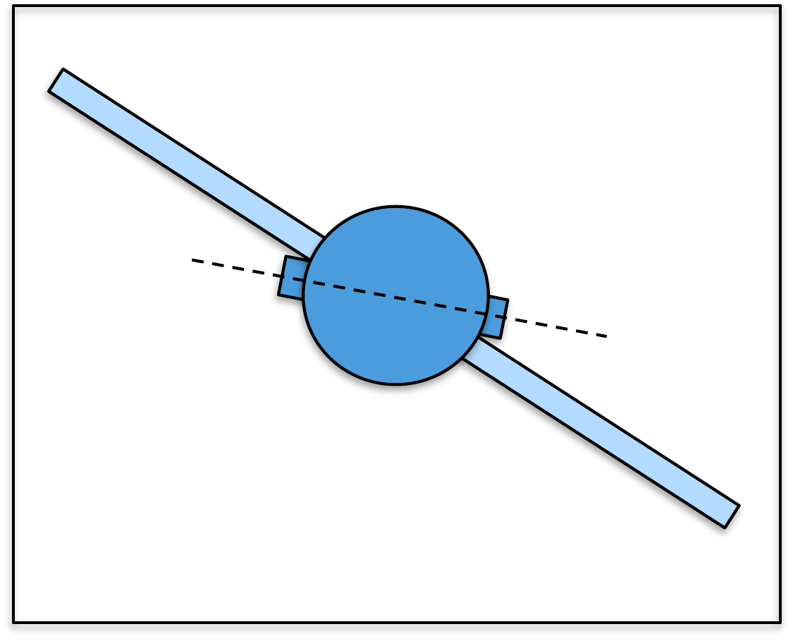
The equations of motion that we derived in the previous section are
often too complicated to facilitate effective engineering design.
Accordingly, the standard approach is to simplify the models into
so-called design models that capture the
essential features of the system. The design techniques studied in this
class will require that the design models are linear and time-invariant.
In addition, the PID method described in
Part III will require that the design
models are second-order systems.
Our approach to developing linear time-invariant design models will
be to linearize the simulation models developed in
Part I and
then to convert the linearized models into two standard forms,
namely
Transfer function models and
State-space models.
Both forms will have advantages and disadvantages that will be
explained throughout the remaining parts of the book. In
Chapter 7 we will define the important
concept of equilibrium and show how the equations of motion can be
linearized about the equilibrium.
Chapter 8 will show how to
transform the linearized equations of motion into transfer function
models, and
Chapter 9 will show how to put the
equations of motion in state-space form.
The remaining parts of the book will use the design models to develop
feedback controllers for the system of interest. In
Part III we will describe the
Proportional-Integral-Derivative (PID) controllers based on second-order
transfer function models.
Part IV derives
observer-based controllers using state-space models. Finally,
Part V describes
loopshaping design strategies using general transfer function
models.
4 Equilibria and Linearization
4.1 Theory
In this chapter we will describe two methods for linearizing the
system, namely Jacobian linearization and feedback
linearization. Jacobian
linearization is based on the idea of approximating the nonlinear terms
in the equations of motion by the first two terms in their Taylor series
expansion. Feedback linearization is based on the idea of using the
input signal to artificially remove the nonlinear terms.
4.1.1 Jacobian Linearization
If the function \(g:\mathbb{R}\to\mathbb{R}\) is a nonlinear
function that can be differentiated an infinite number of times, then
its Taylor series expansion about the
point \(w_0\) is given by \[g(w) = g(w_0) + \left.\frac{\partial g}{\partial
w}\right|_{w_0} (w-w_0) + \frac{1}{2!}\left.\frac{\partial^2 g}{\partial
w^2}\right|_{w_0}(w-w_0)^2 + \cdots.\] A pictorial representation
of Taylor series expansion is shown in
Fig.4.1,
where it can be seen that in a small neighborhood around \(w=w_0\), the function \(g(w)\) is well approximated by the first
two terms in the Taylor series expansion, namely \[g(w)\approx g(w_0) + \left.\frac{\partial
g}{\partial w}\right|_{w_0} (w-w_0).\]
Interactive Figure 4.1
Taylor
series expansion about ω0
Choose a
nonlinear function, move the expansion point, and change the Taylor
polynomial degree. Degree 1 is the linearized model used in Jacobian
linearization.
Figure 4.1. The blue curve is the nonlinear function. The orange curve
is the selected Taylor polynomial about ω0. The
dashed black line shows the first-order term used for
linearization.
Taylor representation
Status:
Symbolic:
Numerical:
Point value:
If \(g\) is a scalar function of
several variables, then the Taylor series about \(w_1=w_{10}, w_2=w_{20}, \cdots,
w_m=w_{m0}\) is given by \[\begin{gathered}
g(w_1,w_2,\dots,w_m) = g(w_{10}, w_{20}, \dots, w_{m0}) +
\left.\frac{\partial g}{\partial
w_1}\right|_{w_{10},w_{20},\dots,w_{m0}} (w_1-w_{10}) \\ +
\left.\frac{\partial g}{\partial
w_2}\right|_{w_{10},w_{20},\dots,w_{m0}} (w_2-w_{20}) + \cdots +
\left.\frac{\partial g}{\partial
w_m}\right|_{w_{10},w_{20},\dots,w_{m0}} (w_m-w_{m0}) + \cdots.
\end{gathered}\] For example, given the function \(g(v,w)=v\cos w\), the constant and linear
terms in the Taylor series, expanded around \(v_0\) and \(w_0\) are \[\begin{aligned}
g(v,w) &\approx g(v_0, w_0)
+ \left.\frac{\partial g}{\partial
v}\right|_{v_{0},w_{0}}(v-v_{0})
+ \left.\frac{\partial g}{\partial
w}\right|_{v_{0},w_{0}}(w-w_{0}) \\
&= v_0\cos w_0 + \left.\left(\cos w
\right)\right|_{v_0,w_0}(v-v_0)
%
+ \left.\left(-v\sin w\right)\right|_{v_0,w_0}(w-w_0) \\
&= v_0\cos w_0 + (\cos w_0)(v-v_0)
- (v_0\sin w_0)(w-w_0).
\end{aligned}\]
Since approximating a nonlinear function by the first two terms in
its Taylor series is only a good approximation in a small neighborhood
of \(w_0\), it is important to select
\(w_0\) judiciously. In particular, we
will be interested in linearizing about equilibrium points of
differential equations.
Given the differential equation \(\dot{x} =
f(x,u)\), the pair \((x_e,u_e)\)
is an equilibrium point if \[f(x_e,u_e)=0.\] In other words, an
equilibrium point is a state-input pair where there is not any motion in
the system.
For example, suppose that the nonlinear differential equation of a
second-order system is given by \[\tag{4.2}
\ddot{y} + a\dot{y} + by + g(y,\dot{y}) = u,\] where \(a\) and \(b\) are constants and \(g(y,\dot{y})\) is a known nonlinear
function of \(y\) and \(\dot{y}\), and \(u\) is the input signal. Defining \(x=(y,\dot{y})^\top\), we get \[\dot{x} = \begin{pmatrix} \dot{y} \\ \ddot{y}
\end{pmatrix}
= \begin{pmatrix} \dot{y} \\ u - a\dot{y} - by - g(y,\dot{y})
\end{pmatrix} \stackrel{\triangle}{=}f(x,u).\] The equilibrium is
when \(f(x_e,u_e)=0\) or in other
words, when \[y_e = \text{~anything~}, \qquad
\dot{y}_e=0, \qquad u_e=by_e+g(y_e,0).\] Equivalently, at
equilibrium there is no motion in the system, which implies that \(\ddot{y}_e=\dot{y}_e=0\), which from
Equation 4.2 implies
that \(u_e = by_e+g(y_e,0)\).
Jacobian linearization then proceeds by
replacing each term in the nonlinear differential equations describing
the system by the first two terms in the Taylor series expansion about
the equilibrium point.
For example, since the first term in
Equation 4.2 is
already linear, it can be expanded exactly as \[\ddot{y} = \ddot{y}_e + \frac{\partial
\ddot{y}}{\partial \ddot{y}}\Big|_e (\ddot{y}-\ddot{y}_e) =
\ddot{\tilde{y}},\] where we have defined the linearized quantity
\(\tilde{y}\stackrel{\triangle}{=}y-y_e\),
and we have used the fact that \(\ddot{y}_e=0\). Similarly, the remaining
terms in
Equation 4.2 are
linearized as \[\begin{aligned}
a\dot{y} &= a\dot{y}_e + a\frac{\partial \dot{y}}{\partial
\dot{y}}\Big|_e (\dot{y}-\dot{y}_e) = a\dot{\tilde{y}} \\
by &= by_e + b\frac{\partial y}{\partial y}\Big|_e (y-y_e) = by_e +
b\tilde{y} \\
g(y,\dot{y}) &\approx g(y_e,\dot{y}_e) + \frac{\partial g}{\partial
y}\Big|_e(y-y_e) + \frac{\partial g}{\partial
\dot{y}}\Big|_e(\dot{y}-\dot{y}_e) \\
&= g(y_e,0) + \frac{\partial g}{\partial y}\Big|_e\tilde{y} +
\frac{\partial g}{\partial \dot{y}}\Big|_e\dot{\tilde{y}} \\
u &= u_e + \frac{\partial u}{\partial u}\Big|_e (u-u_e) = u_e +
\tilde{u}.
\end{aligned}\] Substituting these expressions into
Equation 4.2 the
resulting linearized equations of motion are \[[\ddot{\tilde{y}}] + [a\dot{\tilde{y}}] + [by_e +
b\tilde{y}] + \left[g(y_e,0) + \frac{\partial g}{\partial
y}\Big|_e\tilde{y} + \frac{\partial g}{\partial
\dot{y}}\Big|_e\dot{\tilde{y}}\right] = [u_e + \tilde{u}]\] Using
the equilibrium \(u_e=by_e+g(y_e,0)\)
gives \[\ddot{\tilde{y}} +
\left(a+\frac{\partial g}{\partial \dot{y}}\Big|_e\right)\dot{\tilde{y}}
+ \left(b+\frac{\partial g}{\partial y}\Big|_e\right)\tilde{y} =
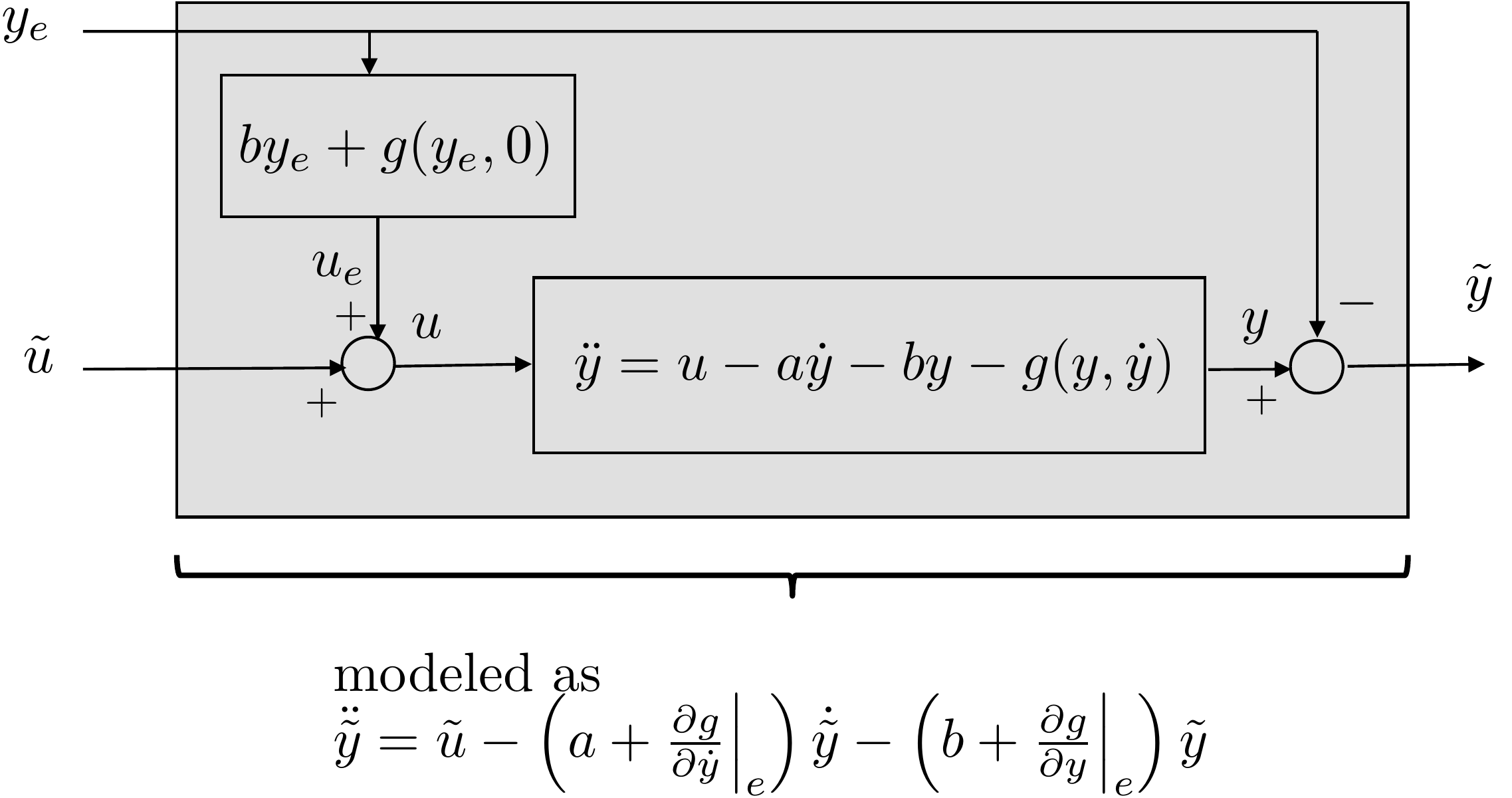
\tilde{u}.\] A block diagram that shows the design model for
Equation 4.2 using
Jacobian linearization is shown in
Fig.4.2.
Figure 4.2. Linear model using Jacobian
linearization.
4.1.2 Feedback Linearization
It is often the case that the nonlinearities in the system can be
directly canceled by a judicious choice for the input variable. Consider
again the nonlinear equations of motion in
Equation 4.2. If
\(u\) is selected as \[u = g(y,\dot{y}) + \tilde{u}\] then the
resulting equation of motion is \[\ddot{y} +
a\dot{y} + by = \tilde{u},\] which is linear. This technique is
called feedback linearization because the feedback
signal \(u\) has been used to linearize
the system by directly canceling the nonlinearities. The advantage of
this method is that the equations of motion are still globally defined
and are not restricted to a small neighborhood of an equilibrium point.
The disadvantage is that \(g(y,\dot{y})\) may not be precisely known,
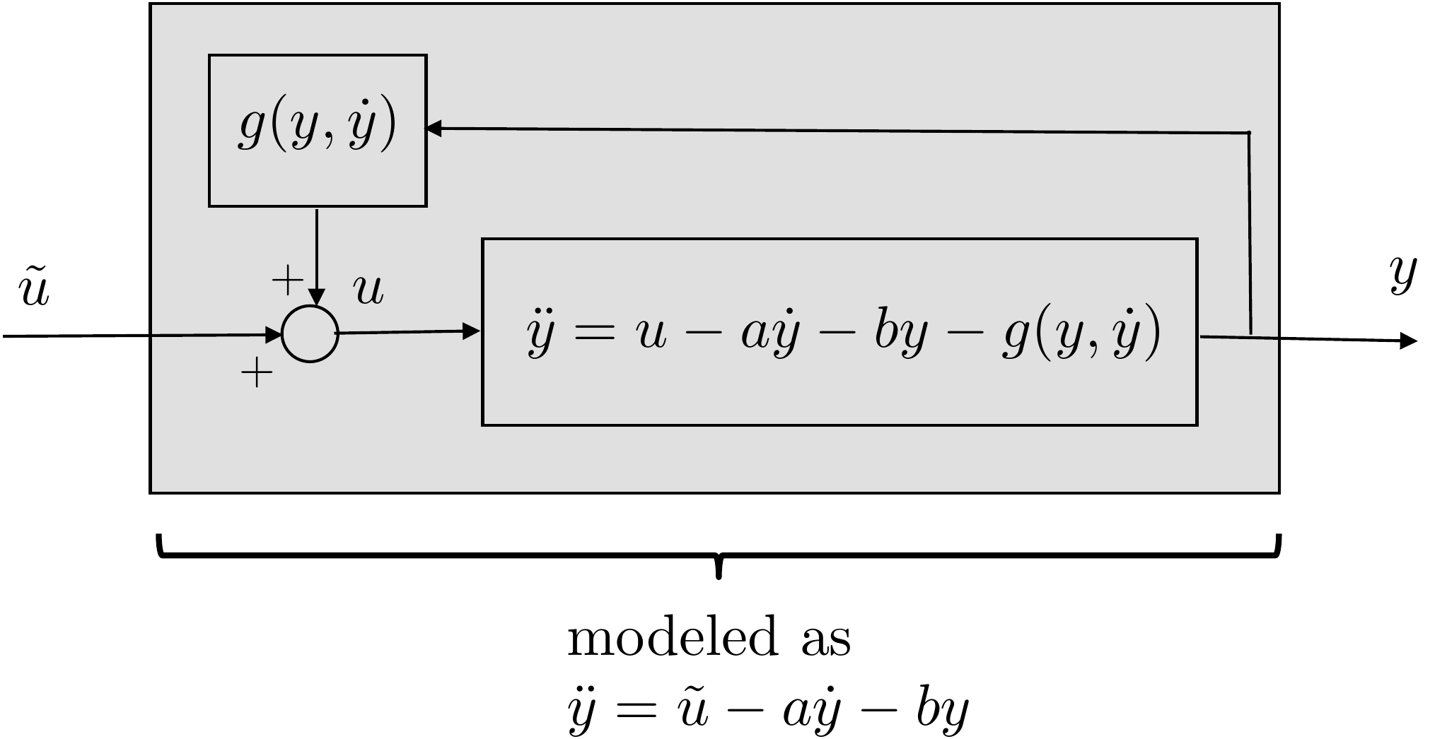
and therefore may not be completely canceled by \(u\). A block diagram that shows the design
model for
Equation 4.2 using
feedback linearization is shown in
Fig.4.3.
Figure 4.3. Linear model using feedback
linearization.
(b) Linearize the system about the equilibria using Jacobian
linearization.
(c) Linearize the system using feedback linearization.
Design Study A guided exercise
Linearize the arm model
Use the nonlinear arm equation
from Chapter 3 and compare Jacobian linearization with feedback
linearization.
Step 1. Equilibrium conditions
Show solution for
Step 1
Answer:\(\dot{\theta}_e=0\) and \(\tau_e=mg\ell\cos\theta_e/2\).
Step
2. Linearized gravity term
Enter the coefficient multiplying
\(\tilde{\theta}\) after
linearizing the gravity torque.
Show solution for Step
2
Answer: The tangent term is
\(-(mg\ell/2)\sin(\theta_e)\tilde{\theta}\).
Step 3.
Feedback-linearizing torque
Show
solution for Step 3
Answer: Use
\(\tau=mg\ell\cos\theta/2+\tilde{\tau}\) so the gravity
term is canceled by the actual angle, not just by the equilibrium
angle.
Complete solution
The differential equation describing the single-link robot arm
derived in HW 3.1.3 is \[\tag{4.3}
\frac{m\ell^2}{3}\ddot{\theta} + \frac{mg\ell}{2}\cos\theta = \tau -
b\dot{\theta}.\] Defining \(x=(\theta,
\dot{\theta})\), and \(u=\tau\)
we get \[\begin{aligned}
\dot{x} = \begin{pmatrix} \dot{\theta} \\ \ddot{\theta}\end{pmatrix}
= \begin{pmatrix} \dot{\theta} \\ \frac{3}{m\ell^2}\tau -
\frac{3b}{m\ell^2}\dot{\theta} - \frac{3g}{2\ell}\cos\theta
\end{pmatrix} \stackrel{\triangle}{=}f(x,u).
\end{aligned}\] The equilibrium is when \(f(x_e,u_e)=0\), or in other words, when
\[\tag{4.4}
\theta_e = \text{~anything~}, \qquad \dot{\theta}_e =0, \qquad \tau_e =
\frac{mg\ell}{2}\cos\theta_e.\] Equivalently, at equilibrium
there is no motion in the system, which implies that \(\ddot{\theta}_e = \dot{\theta}_e=0\), which
from Equation 4.3
implies that \(\tau_e =
\frac{mg\ell}{2}\cos\theta_e\).
Therefore, any pair \((\theta_e,
\tau_e)\) satisfying Equation [dm:arm_equilibrium] is an
equilibrium. Jacobian linearization then proceeds by replacing each term
in the nonlinear differential equations describing the system by the
first two terms in the Taylor’s series expansion about the equilibrium
point. Using some of the relationships from Equation [dm:arm_equilibrium], (such as
\(\dot{\theta}_e = 0\)), then by
defining \(\tilde{\theta}\stackrel{\triangle}{=}\theta-\theta_e\),
\(\dot{\tilde{\theta}}\stackrel{\triangle}{=}\dot{\theta}-\dot{\theta}_e=\dot{\theta}\),
\(\ddot{\tilde{\theta}}=\ddot{\theta}-\ddot{\theta}_e=\ddot{\theta}\),
and \(\tilde{\tau}=\tau-\tau_e\), each
term in Equation 4.3
can be expanded about the equilibrium as follows: \[\begin{aligned}
\frac{m\ell^2}{3}\ddot{\theta} &= \frac{m\ell^2}{3}\ddot{\theta}_e +
\frac{m\ell^2}{3}\left.\frac{\partial \ddot{\theta}}{\partial
\ddot{\theta}}\right|_e (\ddot{\theta}-\ddot{\theta}_e) =
\frac{m\ell^2}{3} \ddot{\tilde{\theta}}, \\
\frac{mg\ell}{2}\cos\theta &\approx \frac{mg\ell}{2} \cos\theta_e +
\frac{mg\ell}{2}\frac{\partial}{\partial \theta}
(\cos\theta)\Big|_{\theta_e}
(\theta-\theta_e) \\
&= \frac{mg\ell}{2}\cos\theta_e - \frac{mg\ell}{2}\sin\theta_e
\tilde{\theta} \\
\tau &= \tau_e + \frac{\partial \tau}{\partial \tau}\Big|_e
(\tau-\tau_e)
= \tau_e + \tilde{\tau} \\
b\dot{\theta} &= b\dot{\theta}_e + b\frac{\partial
\dot{\theta}}{\partial \dot{\theta}}\Big|_e
(\dot{\theta}-\dot{\theta}_e) = b\dot{\tilde{\theta}}.
\end{aligned}\] Substituting into Equation 4.3
gives \[\frac{m\ell^2}{3}\left[\ddot{\theta}_e +
\ddot{\tilde{\theta}}\right] + \frac{mg\ell}{2}\left[\cos\theta_e -
\sin\theta_e\tilde{\theta}\right] = \left[\tau_e+\tilde{\tau}\right] -
b\left[\dot{\theta}_e +\dot{\tilde{\theta}}\right].\] Simplifying
this expression using Equation [dm:arm_equilibrium] gives \[\tag{4.5}
\frac{m\ell^2}{3}\ddot{\tilde{\theta}} -
\frac{mg\ell}{2}(\sin\theta_e)\tilde{\theta} = \tilde{\tau} -
b\dot{\tilde{\theta}},\] which are the linearized equations of
motion using Jacobian linearization.
Feedback linearization proceeds by using the feedback linearizing
control \[\tag{4.6}
\tau = \frac{mg\ell}{2}\cos\theta + \tilde{\tau}\] in Equation 4.3
to obtain the feedback linearized equations of motion \[\tag{4.7}
\frac{m\ell^2}{3}\ddot{\theta} = \tilde{\tau} - b\dot{\theta},\]
where we emphasize that the equations of motion are valid for any \(\theta\) and \(\dot{\theta}\) and not just in a small
region about an equilibrium. It is interesting to compare Equation 4.6
to the control signal using Jacobian linearization which is \[\tag{4.8}
\tau = \tau_e+\tilde{\tau} = \frac{mg\ell}{2}\cos\theta_e +
\tilde{\tau}.\] The control signal in 4.8
uses the equilibrium angle \(\theta_e\)
whereas the control signal in 4.6
uses the actual angle \(\theta\). For
the single-link robot arm we will use the design model obtained using
feedback linearization.
(b) Linearize the system about the equilibria using Jacobian
linearization.
Note that for the inverted pendulum, since the nonlinearities are not
all contained in the same channel as the control force \(F\), the system cannot be feedback
linearized.
Design
Study B guided exercise
Find equilibria and linearization
facts
Check the equilibrium conditions and the key
upright-linearization structure.
Step 1. Equilibrium
conditions
Show solution for Step
1
Answer: At equilibrium F_e = 0
and theta_e = k pi; z_e can be any cart position.
Step
2. Upright linearization
Show solution for Step
2
Answer: For the upright
equilibrium, sin(theta) linearizes to the perturbation
angle.
Step 3. Feedback
linearization
Show solution for Step
3
Answer: The nonlinearities are
not all in the same channel as the cart force, so feedback linearization
is not available in this form.
Complete solution
The differential equations describing the inverted pendulum derived
in HW 3.2.3 are \begin{align}
(m_1+m_2)\ddot{z} + m_1 \frac{\ell}{2} \ddot{\theta} \cos\theta &=
m_1 \frac{\ell}{2} \dot{\theta}^2\sin\theta -b\dot{z} + F
\tag{4.9} \\
m_1 \frac{\ell}{2} \ddot{z} \cos\theta + m_1 \frac{\ell^2}{3}
\ddot{\theta} &=
m_1 g \frac{\ell}{2} \sin\theta. \notag
\end{align} The equilibrium values \((z_e,\theta_e,F_e)\) are found by setting
\(\dot{z}=\ddot{z}=\dot{\theta}=\ddot{\theta}=0\)
in Equation 4.9
to obtain \begin{align}
F_e &= 0 \tag{4.10} \\
m_1g\frac{\ell}{2}\sin\theta_e &=
0.\tag{4.11}
\end{align} Therefore, any triple \((z_e, \theta_e, F_e)\) satisfying
Equations 4.10
and 4.11
is an equilibrium. In other words, \(z_e\) can be any value, \(F_e=0\), and \(\theta_e = k\pi\), where \(k\) is an integer.
To linearize around \((z_e, \theta_e,
F_e)\) where \(k\) is an even
integer, note that \[\begin{aligned}
\ddot{\theta}\cos\theta &\approx
\ddot{\theta}_e\cos\theta_e
+
\frac{\partial}{\partial\theta}(\ddot{\theta}\cos\theta)\Big|_{(\ddot{\theta}_e,\theta_e)}(\theta-\theta_e)
%
+
\frac{\partial}{\partial\ddot{\theta}}(\ddot{\theta}\cos\theta)\Big|_{(\ddot{\theta}_e,\theta_e)}(\ddot{\theta}-\ddot{\theta}_e)
\\
&= \ddot{\theta}_e\cos\theta_e
- (\ddot{\theta}_e\sin\theta_e)\tilde{\theta}
+ (\cos\theta_e)\ddot{\tilde{\theta}} \\
&= \ddot{\tilde{\theta}} \\
%
\dot{\theta}^2\sin\theta &\approx \dot{\theta}_e^2\sin\theta_e +
\frac{\partial}{\partial\theta}(\dot{\theta}^2\sin\theta)\Big|_{(\theta_e,\dot{\theta}_e)}(\theta-\theta_e)
%
+
\frac{\partial}{\partial\dot{\theta}}(\dot{\theta^2}\sin\theta)\Big|_{(\theta_e,\dot{\theta}_e)}(\dot{\theta}-\dot{\theta}_e)
\\
&= \dot{\theta}_e^2\sin\theta_e +
\dot{\theta}_e^2\cos\theta_e\tilde{\theta} +
2\dot{\theta}_e\sin\theta_e\dot{\tilde{\theta}} \\
&= 0, \\
%
\ddot{z}\cos\theta &\approx
\ddot{z}_e\cos\theta_e
+
\frac{\partial}{\partial\theta}(\ddot{z}\cos\theta)\Big|_{(\ddot{z}_e,\theta_e)}(\theta-\theta_e)
%
+
\frac{\partial}{\partial\ddot{z}}(\ddot{z}\cos\theta)\Big|_{(\ddot{z}_e,\theta_e)}(\ddot{z}-\ddot{z}_e)
\\
&= \ddot{z}_e\cos\theta_e
- (\ddot{z}_e\sin\theta_e)\tilde{\theta}
+ (\cos\theta_e)\ddot{\tilde{z}} \\
&= \ddot{\tilde{z}} \\
%
\sin\theta &\approx \sin\theta_e + \frac{\partial}{\partial \theta}
(\sin\theta)\Big|_{\theta_e}
(\theta-\theta_e) \\
&= \sin\theta_e + (\cos\theta_e) \tilde{\theta} \\
&= \tilde{\theta},
\end{aligned}\] where we have defined \(\tilde{\theta}\stackrel{\triangle}{=}\theta-\theta_e\)
and \(\tilde{z}\stackrel{\triangle}{=}z-z_e\).
Also defining \(\tilde{F}\stackrel{\triangle}{=}F-F_e\),
and noting that \[\begin{aligned}
\theta &= \theta_e + \tilde{\theta} = \tilde{\theta} \\
\dot{\theta} &= \dot{\theta}_e + \dot{\tilde{\theta}} =
\dot{\tilde{\theta}} \\
z &= z_e + \tilde{z} \\
\dot{z} &= \dot{z}_e + \dot{\tilde{z}} = \dot{\tilde{z}} \\
\ddot{z} &= \ddot{z}_e + \ddot{\tilde{z}} = \ddot{\tilde{z}} \\
F &= F_e + \tilde{F} = \tilde{F},
\end{aligned}\] we can write Equation 4.9
in its linearized form as \[\begin{aligned}
(m_1+m_2)[\ddot{z}_e+\ddot{\tilde{z}}] + m_1 \frac{\ell}{2}
[\ddot{\tilde{\theta}}] &=
m_1 \frac{\ell}{2} [ 0 ] -b[\dot{z}_e+\dot{\tilde{z}}] +
[F_e+\tilde{F}]
\\
m_1 \frac{\ell}{2} [ \ddot{\tilde{z}}] + m_1 \frac{\ell^2}{3}
[\ddot{\theta}_e+\ddot{\tilde{\theta}}] &=
m_1 g \frac{\ell}{2} [\tilde{\theta}],
\end{aligned}\] which simplifies to \[\tag{4.12}
\begin{pmatrix} (m_1+m_2) & m_1 \frac{\ell}{2} \\
m_1 \frac{\ell}{2} & m_1 \frac{\ell^2}{3}
\end{pmatrix}\begin{pmatrix}
\ddot{\tilde{z}} \\ \ddot{\tilde{\theta}} \end{pmatrix} =
\begin{pmatrix} -b\dot{\tilde{z}} + \tilde{F}
\\
m_1 g \frac{\ell}{2} \tilde{\theta} \end{pmatrix},\] which
are the linearized equations of motion.
Defining \(x=(\theta, \phi, \dot{\theta},
\dot{\phi})\), and \(u=\tau\) we
get \[\begin{aligned}
\dot{x} = \begin{pmatrix} \dot{\theta} \\ \dot{\phi} \\ \ddot{\theta} \\
\ddot{\phi}\end{pmatrix}
= \begin{pmatrix} \dot{\theta} \\ \dot{\phi} \\
-\frac{b}{J_s}(\dot{\theta}-\dot{\phi})
-\frac{k}{J_s}(\theta-\phi)+\frac{1}{J_s}\tau \\ -
\frac{b}{J_p}(\dot{\phi}-\dot{\theta})-\frac{k}{J_p}(\phi-\theta)
\end{pmatrix} \stackrel{\triangle}{=}f(x,u).
\end{aligned}\] The equilibrium is when \(f(x_e,u_e)=0\), or in other words when
\[\tag{4.15}
\theta_e = \phi_e = \text{~anything~}, \qquad \dot{\theta}_e =
\dot{\phi}_e =0, \qquad \tau_e = 0.\]
The equations of motion for this system are linear and do not require
linearization. With that said, the information about the system
equilibria can be helpful for designing the control system. In this
case, understanding that the commanded angular position of the satellite
and the panel should be the same to keep the system in equilibrium will
influence our control design.
4.5 Interactive Linearization
Check
Chapter 4 activity
Local linear model of a nonlinear equation
Use f(x,u)=x2+u to compare the nonlinear surface, the
selected operating point, the tangent-plane linearization, and the
approximation error.
Interactive Figure 4.I2. The blue mesh is the nonlinear surface f(x,u).
The orange mesh is the tangent plane at (x0, u0).
Interactive Figure 4.I3. Heat map of approximation error
f(x,u)-flin(x,u). Darker cells indicate larger local
linearization error.
\(f_{\mathrm{lin}}(x,u)\) at the nearby
point = ; true \(f(x,u)\) =
; error =
Notice that the error is small near \(x_0\) and grows as the nearby point moves away from the
linearization point.
A linearized perturbation model is most meaningful when the operating
point is an equilibrium and the perturbation stays near that point.
4.6 Knowledge Check
Q1. Valid region
When is a Jacobian linearization usually the best
approximation?
Q2. Equilibrium condition
For xdot=f(x,u), what condition defines an
equilibrium point?
Q3. Jacobian entry
For f(x,u)=x2+u, enter A =
∂f⁄∂x evaluated
at xe=2.
Show solution
Answer: 4, because
∂f⁄∂x = 2x and
2(2)=4.
Q4. Equilibrium input
For f(x,u)=x2+u and xe=3, enter the input
ue that makes f(xe,ue) = 0.
Show solution
Answer: -9, because 32+ue=0.
Q5. Perturbation variables
In words, what do variables like x-xe represent in a
linearized model?
Show solution
Answer: They are deviations, or perturbations, from the
equilibrium value.
Q6. Equilibrium pair
For the
scalar model xdot = f(x,u) = x2 + u, which pair is an
equilibrium?
Q7. Jacobian entry
For
f2(x,u)=x22+u, what is
A22 = partial f2/partial x2
at x2e = -1?
Q8. Perturbation variable
In a linearized model, what does x -
xe represent?
Q9. Local approximation
Which statement about a Jacobian linearization is
most accurate?
4.7 Notes and References
Jacobian linearization is a standard technique that is well
documented in most introductory textbooks on control. For example,
see [4–7]. Feedback linearization is a much deeper topic
than can be covered in an introductory textbook on control. A discussion
that is similar to ours, that assumes that the nonlinearity is in the
input channel, is contained in [5]. Feedback linearization is a fairly
standard technique for fully actuated mechanical systems modeled by
Euler-Lagrange equations, where the model of the system can be reduced
to \[M(q)\ddot{q} + c(q,\dot{q})\dot{q}+g(q)
= \tau,\] where \(q\in\mathbb{R}^m\) is the generalized
coordinate and \(\tau\in\mathbb{R}^m\)
is the generalized force, and where \(M(q)\) is an invertible matrix. In that
case we can write \[\ddot{q} =
M^{-1}(q)\left(\tau - c(q,\dot{q})\dot{q} - g(q)\right).\]
Selecting \(\tau\) as \[\tag{4.16}
\tau = c(q,\dot{q})\dot{q} + g(q) + M(q)\nu,\] results in the
linear system \[\ddot{q} = \nu,\]
where the new control variable \(\nu\)
can be designed to stabilize the system. The control law in
Equation 4.16
is the feedback linearizing control. This is a standard technique for
robot manipulators and is often called the method of computed
torque [8–10].
When the nonlinearity is not in the input channel, the system can
still often be feedback linearized through a suitable change of
variables. A good introduction to the topic is contained in [11]. More
advanced coverage of the topic can be found in [12–15].