P.1 Simulating Control Systems Using Python
In this appendix we will show how to simulate the feedback control of
a dynamic system using Python. Consider the general
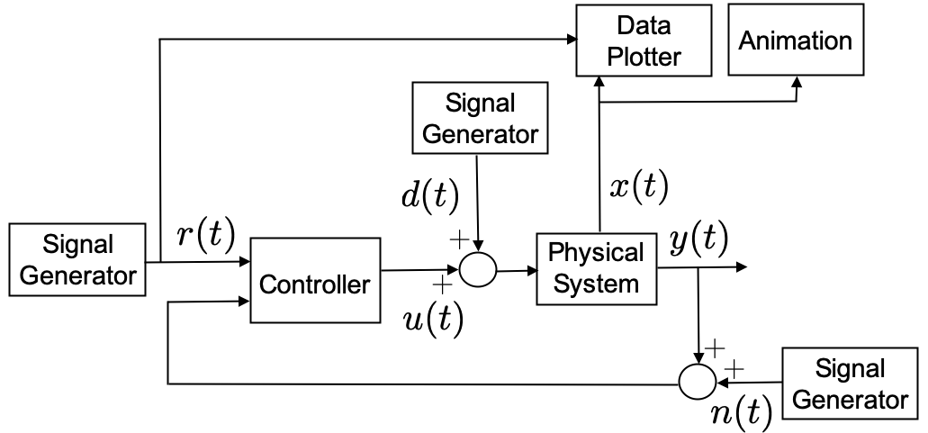
feedback control system shown in
Figure 1.1. The output
of the physical system is \(y(t)\), and
the input to the physical system is \(u(t)\) plus an external disturbance signal
\(d(t)\). The output of the system is
corrupted by zero-mean noise \(n(t)\).
The input to the controller is the reference signal \(r(t)\) as well as the output corrupted by
noise. In Python, each block shown in
Figure 1.1 is
implemented using a Python class.
We will illustrate how to implement feedback control systems in
Python by simulating the physical system described by the
differential equation \[\tag{P.1.1}
\ddot{y} + 2\dot{y} + 3 y = 4 u,\] and using the PID controller
\[\tag{P.3.2}
u(t) = k_p (r(t)-y(t)) + k_i \int_{-\infty}^t (r(\tau)-y(\tau))d\tau -
k_d \dot{y}.\]
The feedback control system shown in
Figure 1.1 is simulated
in systemSim.py, which is listed below.
import matplotlib.pyplot as plt
from systemDynamics import systemDynamics
from systemController import systemController
from signalGenerator import signalGenerator
from systemAnimation import systemAnimation
from dataPlotter import dataPlotter

# simulation parameters
t_start = 0.0  # start time
t_end = 20.0  # end time
t_plot = 0.1  # sample rate for plotter and animation
Ts = 0.01  # sample rate for dynamics and controller

# instantiate system, controller, and reference classes
system = systemDynamics(sample_rate=Ts)
controller = pendulumController(sample_rate=Ts)
reference = signalGenerator(amplitude=0.5, frequency=0.05)
disturbance = signalGenerator(amplitude=1.0, frequency = 0.0)
noise = signalGenerator(amplitude=0.01)

# instantiate the simulation plots and animation
dataPlot = dataPlotter()
animation = systemAnimation()

t = t_start  # time starts at t_start
y = system.h()  # output of system at start of simulation
while t < t_end:  # main simulation loop
    # set time for next plot
    t_next_plot = t + t_plot
    # Propagate dynamics and controller at fast rate Ts
    while t < t_next_plot:
        r = reference.square(t)  # assign reference
        d = disturbance.step(t)  # simulate input disturbance
        n = noise.random(t)  # simulate sensor noise
        u = controller.update(r, y + n)  # update controller
        y = system.update(u + d)  # Propagate the dynamics
        t = t + Ts  # advance time by Ts
    # update animation and data plots
    animation.update(system.state)
    dataPlot.update(t, ref_input, pendulum.state, u)
    # pause causes the figure to be displayed during the simulation
    plt.pause(0.0001)

# Keeps the program from closing until the user presses a button.
print('Press key to close')
plt.waitforbuttonpress()
plt.close()
The physical system is implemented in a class contained in
systemDynamic.py, which will be discussed below, and which
is imported on line 2, and instantiated on line 15. The system is
updated at sample rate \(T_s\) given
the control input \(u\) and the input
disturbance \(d\) on line 36.
The controller is implemented in a class contained in
systemController.py, which will be discussed below, and
which is imported on line 3, and instantiated on line 16. Given the
reference input \(r\), and the system
output \(y\), the controller is updated
at the fast sample rate \(T_s\) on
line 35. At the initial time, the controller needs the initial output at
time \(t=0\), which is computed on
line 26 before the main loop begins.
The reference input is implemented using the
signalGenerator class that is contained in
signalGenerator.py, which is described below and imported
on line 4 and instantiated on line 17. The reference input at time \(t\), i.e., \(r(t)\), is assigned a value on line 32.
The external disturbance \(d(t)\) is
also implemented using the
signalGenerator class and is instantiated on line 17, and
assigned a value on line 33. For this example, the external disturbance
will be a constant value of \(d(t)=1.0\). The disturbance is assigned on
line 33, and is input to the system on line 36.
In addition to the feedback loop implemented above, the system will
be visualized through an animation and by plotting important variables
such as the reference input, the system states, and the control input.
The animation and data plotting functions are implemented in
systemAnimation.py and
dataPlotter.py, imported on lines 5 and 6, instantiated on
lines 22 and 23, and updated on lines 39 and 40. The pause
command on line 42 forces the animation and data plotting functions to
update their displays each time through the loop.
P.1.1 System Dynamics
This section will describe how to implement the system dynamics given in Equation P.1.1. The first step is to convert the dynamics to the state-space form \[\begin{aligned} \dot{x} &= f(x, u) \\ y &= h(x,u). \end{aligned}\] For the differential equation in Equation P.1.1 let \(x = (y, \dot{y})^\top\), which gives \begin{align} \dot{x}& = \begin{pmatrix} \dot{x}_1 \\ \dot{x}_2 \end{pmatrix} = \begin{pmatrix} \dot{y} \\ \ddot{y} \end{pmatrix} = \begin{pmatrix} \dot{y} \\ -2\dot{y} - 3y + 4u \end{pmatrix} = \begin{pmatrix} x_2 \\ -2x_2 - 3 x_1 + 4 u \end{pmatrix} \stackrel{\triangle}{=}f(x,u) \tag{P.1.3} \\ y &= x_1 \stackrel{\triangle}{=}h(x). \tag{P.1.4} \end{align}
The dynamics of the system are implemented in
systemDynamics.py, which is listed below.
import numpy as np

class systemDynamics:
    def __init__(self, sample_rate):
        # Initial state conditions
        y0 = 0.0
        ydot0 = 0.0
        self.state = np.array([
            [y0],  # initial condition for y
            [ydot0],  # initial condition for ydot
        ])
        self.Ts = sample_rate  # sample rate of system
        self.limit = 1.0  # input saturation limit
        # system parameters
        self.a0 = 3.0
        self.a1 = 2.0
        self.b0 = 4.0
        # modify the system parameters by random value
        alpha = 0.2  # Uncertainty parameter
        self.a1 = self.a1 * (1.+alpha*(2.*np.random.rand()-1.))
        self.a0 = self.a0 * (1.+alpha*(2.*np.random.rand()-1.))
        self.b0 = self.b0 * (1.+alpha*(2.*np.random.rand()-1.))

    def f(self, state, u):
        # for system xdot = f(x,u), return f(x,u)
        y = state.item(0)
        ydot = state.item(1)
        # The equations of motion.
        yddot = -self.a1 * ydot - self.a0 * y + self.b0 * u
        # build xdot and return
        xdot = np.array([[ydot], [yddot]])
        return xdot

    def h(self):
        # Returns the measured output y = h(x)
        y = self.state.item(0)
        # return output
        return y

    def update(self, u):
        # This is the external method that takes the input u(t)
        # and returns the output y(t).
        u = self.saturate(u, self.limit)  # saturate the input
        self.rk4_step(u)  # propagate the state by one time step
        y = self.h()  # compute the output at the current state
        return y

    def rk4_step(self, u):
        # Integrate ODE using Runge-Kutta RK4 algorithm
        F1 = self.f(self.state, u)
        F2 = self.f(self.state + self.Ts / 2 * F1, u)
        F3 = self.f(self.state + self.Ts / 2 * F2, u)
        F4 = self.f(self.state + self.Ts * F3, u)
        self.state += self.Ts / 6 * (F1 + 2 * F2 + 2 * F3 + F4)

    def saturate(self, u, limit):
        if abs(u) > limit:
            u = limit*np.sign(u)
        return u
The system is initialized in lines 4–22. The state is initialized in
lines 6–11 based on the initial conditions for \(y(0)\) and \(\dot{y}(0)\). The system parameters are
initialized in lines 15–22. The parameters for any physical system are
never known exactly. Therefore, feedback systems need to be designed to
be robust to this uncertainty. In the simulation, we model uncertainty
in our knowledge of the physical parameters by changing the nominal
value by a uniform random variable. Let \(\alpha\) be the amount of change allowed
for each parameter. For example, \(\alpha =
0.2\) means that the physical parameters may change by up to 20%.
The function np.random.rand() returns a uniform random
variable in the interval \([0, 1]\).
Therefore, \((1 + \alpha
(2*\texttt{np.random.rand()}-1))\) is a random variable in the
interval \([-\alpha, \alpha]\). The
nominal values for the physical parameters that are known to the
designer are specified in lines 15–17. The actual values used by the
simulation are randomly selected in lines 19–22.
The system dynamics \[\begin{aligned} \dot{x} &= f(x, u) \\ y &= h(x, u). \end{aligned}\] are specified in lines 24–38. Lines 24–32 define \(f(x,u)\), and lines 34–38 define \(h(x, u)\), as given by Equations P.1.3 and P.1.4 respectively.
The main feedback loop calls the update routine in
lines 40–46. The update function first saturates the input
in line 43, where the saturation function is defined in
lines 56–59. The system dynamics are then propagated forward by one
sample time \(T_s\) using the
fourth-order Runge-Kutta algorithm in line 44, where the RK4 algorithm
is specified in lines 48–54, as described in
Appendix 28. The update
function finally computes and returns the output \(y\) in lines 45–46.
P.1.2 Controller
This section will describe how to implement the PID controller given
in Equation P.3.2. The
controller is implemented in systemController.py, which is
listed below.
import numpy as np

class systemController:
    def __init__(self, sample_rate):
        # specify gains
        self.kp = 1.0
        self.kd = 1.0
        self.ki = 1.0
        self.Ts = sample_rate
        self.sigma = 2.0 * self.Ts
        self.beta = (2.0*sigma-self.Ts)/(2.0*sigma+self.Ts)
        self.limit = 1.0
        # internal storage for differentiator
        self.y_dot = 0.0
        self.y_d1 = 0.0
        # internal storage for integrator
        self.integrator = 0
        self.error_d1 = 0

    def update(self, r, y):
        e = r - y  # define the error
        I = self.integrate_e(e)  # integrate error
        ydot = self.differentiate_y(y)  # differentiate y
        # form PID controller, saturate, and return
        u = self.kp * e + self.ki * I - self.kd * ydot
        u = self.saturate(u)
        return u

    def integrate_e(self, e):
        self.integrator = self.integrator
            + (self.Ts / 2) * (error + self.error_d1)
        self.error_d1 = error
        return self.integrator

    def differentiate_y(self, y):
        self.y_dot = self.beta*self.y_dot
            + (1-self.beta)/self.Ts * (y - self.y_d1)
        self.y_d1 = y
        return self.y_dot

    def saturate(self, u):
        if abs(u) > self.limit:
            u = self.limit*np.sign(u)
        return u
The controller is instantiated in lines 4–18. The PID gains are
specified in lines 6–8. The sample rate of the controller is passed into
the system at the time of instantiation and is assigned an internal
variable \(T_s\) in line 9. The dirty
derivative gain \(\sigma\), described
in
Chapter 13, is specified in
line 10, and the intermediate gain \(\beta =
\frac{2\sigma-T_s}{2\sigma+T_s}\) is specified on line 11.
Internal storage variables for the differentiator and the integrator, as
explained in
Chapter 13, are given in
lines 13–18. The PID control update routine is specified in
lines 20–27. The error \(e=r-y\), as
shown in
Figure 1.1, is defined
in line 21. The PID controller in
Equation P.3.2 uses
the integral of \(e\) and the
derivative of \(y\). The integral of
\(e\) is computed on line 22 using the
routine specified in lines 29–33. A derivation of the integral equations
is given in
Chapter 13. The derivative
of \(y\) is computed in line 23 using
the routine specified in lines 35–39. A derivation of the dirty
derivative equations is given in
Chapter 13. Finally, the
PID controller is computed, the value is saturated, and the result is
returned in lines 25, 26, and 27, respectively.
P.1.3 Signal Generator
Python code for the signal generator class is listed below.
import numpy as np

class signalGenerator:
    def __init__(self, amplitude=1.0, frequency=0.001, y_offset=0):
        self.amplitude = amplitude  # signal amplitude
        self.frequency = frequency  # signal frequency
        self.y_offset = y_offset  # signal y-offset

    def square(self, t):
        if t % (1.0/self.frequency) <= 0.5/self.frequency:
            out = self.amplitude + self.y_offset
        else:
            out = - self.amplitude + self.y_offset
        return out

    def sawtooth(self, t):
        tmp = t % (0.5/self.frequency)
        out = 4 * self.amplitude * self.frequency*tmp
              - self.amplitude + self.y_offset
        return out

    def step(self, t):
        if t >= 0.0:
            out = self.amplitude + self.y_offset
        else:
            out = self.y_offset
        return out

    def random(self, t):
        out = np.random.normal(self.y_offset, self.amplitude)
        return out

    def sin(self, t):
        out = self.amplitude * np.sin(2*np.pi*self.frequency*t)
              + self.y_offset
        return out
The class is instantiated by passing in the desired amplitude of the signal, the frequency in Hertz, and a y-offset value. For random signals, the amplitude is interpreted to be the standard deviation of the signal. The signal generator can then be used to produce a square wave, a sawtooth signal, a step, a random signal, or a sinusoid, as specified in lines 9–36.
P.1.4 Data Plotter
The objective of the data plotter is to plot the relevant signals
during the simulation. For this simple example, we will plot the output
\(y\) and the reference \(r\) on one plot, the velocity \(\dot{y}\) on another plot, and the control
signal \(u\) on a third plot. For
plotting and animation, we will use the Python Matplotlib
library. Python code for the data plotter class is listed below.
import matplotlib.pyplot as plt
from matplotlib.lines import Line2D
import numpy as np

plt.ion()  # enable interactive drawing

class dataPlotter:
    def __init__(self):
        # Number of subplots = num_of_rows*num_of_cols
        self.num_rows = 3    # Number of subplot rows
        self.num_cols = 1    # Number of subplot columns
        # Crete figure and axes handles
        self.fig, self.ax = plt.subplots(self.num_rows,
                                         self.num_cols,
                                         sharex=True)
        # Instantiate lists to hold the time and data histories
        self.time_history = []  # time
        self.r_history = []  # reference r
        self.y_history = []  # output y
        self.ydot_history = []  # velocity ydot
        self.u_history = []  # input u
        # create a handle for every subplot.
        self.handle = []
        self.handle.append(subplotWindow(self.ax[0],
                                  ylabel='y',
                                  title='Simple System'))
        self.handle.append(subplotWindow(self.ax[1],
                                  ylabel='ydot'))
        self.handle.append(subplotWindow(self.ax[2],
                                  xlabel='t(s)',
                                  ylabel='u'))

    def update(self, time, reference, state, control):
        # update the time history of all plot variables
        self.time_history.append(time)
        self.r_history.append(reference)
        self.y_history.append(state.item(0))
        self.ydot_history.append(state.item(1))
        self.u_history.append(control)

        # update the plots with associated histories
        self.handle[0].update(self.time_history,
                              [self.r_history, self.y_history])
        self.handle[1].update(self.time_history,
                              [self.ydot_history])
        self.handle[2].update(self.time_history,
                              [self.u_history])

class subplotWindow:
    # Create each individual subplot.
    def __init__(self, ax, xlabel='', ylabel='', title='',
                 legend=None):
        '''
            ax - This is a handle to the  axes of the figure
            xlabel - Label of the x-axis
            ylabel - Label of the y-axis
            title - Plot title
            legend - A tuple of strings that identify the data.
                     EX: ("data1","data2", ... , "dataN")
        '''
        self.legend = legend
        self.ax = ax                  # Axes handle
        self.colors = ['b', 'g', 'r', 'c', 'm', 'y', 'b']
        # A list of colors. The first color in the list corresponds
        # to the first line object, etc.
        # 'b' - blue, 'g' - green, 'r' - red, 'c' - cyan,
        # 'm' - magenta, 'y' - yellow, 'k' - black
        self.line_styles = ['-', '-', '--', '-.', ':']
        # A list of line styles.  The first line style in the list
        # corresponds to the first line object.
        # '-' solid, '--' dashed, '-.' dash_dot, ':' dotted
        self.line = []
        # Configure the axes
        self.ax.set_ylabel(ylabel)
        self.ax.set_xlabel(xlabel)
        self.ax.set_title(title)
        self.ax.grid(True)
        # Keeps track of initialization
        self.init = True

    def update(self, time, data):
        # Adds data to the plot.
        # Initialize the plot the first time routine is called
        if self.init==True:
            for i in range(len(data)):
                # Instantiate line object and add it to the axes
                self.line.append(Line2D(time, data[i],
                    color=self.colors[np.mod(i,len(self.colors)-1)],
                    ls=self.line_styles
                            [np.mod(i, len(self.line_styles) - 1)],
                    label=self.legend
                        if self.legend!=None else None))
                self.ax.add_line(self.line[i])
            self.init = False
            # add legend if one is specified
            if self.legend!=None:
                plt.legend(handles=self.line)
        else: # Add new data to the plot
            # Updates the x and y data of each line.
            for i in range(len(self.line)):
                self.line[i].set_xdata(time)
                self.line[i].set_ydata(data[i])

        # Adjusts the axis to fit all of the data
        self.ax.relim()
        self.ax.autoscale()
The plotter is initialized in lines 9–31. Lines 10–11 specify that
the plot window will contain three plots arranged as a \(3\times 1\) array. The routine keeps track
of the time histories of all variables to be plotted. Lines 17–21
initialize time histories for the time \(t\), the reference signal \(r\), the output \(y\), the velocity \(\dot{y}\), and the input \(u\). Lines 23–31 set up the individual
plots with labels by instantiating objects from the
subplotWindow class, which will be described below.
The update method receives as input the current
time,
reference, state, and control
values. Lines 35–39 append the current values to the history lists
maintained in memory for each of those values. The plots are then
updated with the new histories in lines 42–47 by calling the
subplotWindow.update method, which will be described
below.
The subplotWindow class is instantiated in lines 50–79.
If multiple data streams are on a single plot, the color of the line
corresponds to the order specified on line 63, and the style of the
lines will be in the order specified on line 68. The
subplotWindow.update method is specified in lines 81–102.
The first time the subplotWindow.update method is called,
the line objects are initialized and plotted in lines 85–97. In
subsequent calls to subplotWindow.update the data lines are
modified in lines 100–102.
P.1.5 Animation
In this section we will show how to create an animation for the inverted pendulum case study. Consider the image of the inverted pendulum shown in Fig. 1.2, where the configuration is completely specified by the position of the cart \(z\) and the angle of the rod from vertical \(\theta\). The physical parameters of the system are the rod length \(\ell\), the base width \(w\), the base height \(h\), and the gap between the base and the track \(g\).
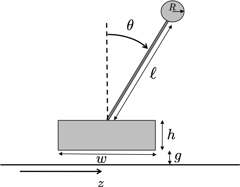
The first step in developing the animation is to determine the position of points that define the animation. The pendulum will require that we draw three objects: the rectangular cart, the circular bob at the end of the rod, and the rod. We will draw the cart as a rectangle, the bob as a circle, and the rod as a line. In Python, rectangles are specified by their lower-left corner, their width, and their height. The lower left corner of the rectangle is \((z-w/2, g)\). In Python, circles are specified by their center and radius. The center of the bob is \((z+(\ell+R)\sin\theta, g+h+(\ell+R)\cos\theta)\). In Python, lines are specified by the \(x\) and \(y\) locations of their endpoints. The \(x\) locations of the endpoints of the rod are \(X=(z, z+\ell\sin\theta)\), and the \(y\) locations of the endpoints are \(Y=(g+h, g+h+\ell\cos\theta)\).
Python code for the animation class is listed below.
# 3rd-party
import numpy as np
import matplotlib.patches as mpatches

# local (controlbook)
from ..common.animator import MatplotlibAxisAnimator


class CartPendulumAnimator(MatplotlibAxisAnimator):
    def setup_background(self):
        self.color = "blue"

        self.length = 1.0
        self.cart_width = self.length / 2
        self.cart_height = self.length * 0.15
        self.gap = 0.01
        self.buffer = self.length * 3

        span = 10
        (groundline,) = self.ax.plot([-span, span], [0, 0], "k--")

        z0 = self.x_hist[0, 0]
        self.ax.grid(True)
        self.ax.set_aspect("equal", "box")
        self.ax.set_xlim(z0 - self.buffer, z0 + self.buffer)
        self.ax.set_ylim(-self.buffer / 2, self.buffer)

    def setup_changing_objects(self, x0, r0):
        z0, theta0 = x0[:2]
        bottom_left_corner = self.get_cart_corner(z0)
        self.cart = mpatches.Rectangle(
            xy=bottom_left_corner,
            width=self.cart_width,
            height=self.cart_height,
            rotation_point="xy",
            facecolor=self.color,
            edgecolor="black",
        )
        self.ax.add_patch(self.cart)

        x, y = self.get_pendulum_data(z0, theta0)
        (self.pendulum,) = self.ax.plot(x, y, lw=1, c=self.color)
        (self.bob,) = self.ax.plot(x[-1:], y[-1:], "o", c=self.color)

    def update_changing_objects(self, x, r):
        z, theta = x[:2]

        bottom_left_corner = self.get_cart_corner(z)
        self.cart.set_xy(bottom_left_corner)

        x, y = self.get_pendulum_data(z, theta)
        self.pendulum.set_data(x, y)
        self.bob.set_data(x[-1:], y[-1:])
        return (self.cart, self.pendulum, self.bob)

    def get_cart_corner(self, z):
        bottom_left = (z - self.cart_width / 2, self.gap)
        return bottom_left

    def get_pendulum_data(self, z, theta):
        bottom = self.gap + self.cart_height
        x = [z, z + self.length * np.sin(theta)]
        y = [bottom, bottom + self.length * np.cos(theta)]
        return x, y
The pendulumAnimation class is initialized in
lines 7–18. The flag self.flag_init is used to indicate the
first time the animation function is called. On the first call when
self.flag_init==True, all of the plot elements are
initialized and configured (see lines 38–45, lines 55–62, and
lines 71–75). After the first call, when
self.flag_init==False, each plot element is simply updated
(see lines 47, lines 64, and lines 77–78). Line 10 initializes the plot
window and axes, line 12 initializes an empty list of handles to plot
objects, line 14 sets the size of the axes to be \(\pm 3\ell\) along the \(x\)-axis and \(-0.1\) to \(3\ell\) along the \(y\)-axis, line 16 draws the line
representing the ground, and line 18 labels the \(x\)-axis as the configuration variable
\(z\).
The animation function is updated each time step using the
update method shown in lines 20–30. The input to the
update method is the state of the pendulum, of
which the first element is \(z\) and
the second element is \(\theta\)
(lines 21–22). Lines 24–26 then call methods that will be described
below and that draw the cart, bob, and rod. Line 27 ensures that the
axes are not distorted. Lines 29–30 set the initialization flag
self.flat_init to False after the first call
to update.
The draw_cart method is listed in lines 32–47. The cart
is drawn as a rectangle patch, which is specified by its lower-left
corner and the width and height of the rectangle. The lower-left corner
of the rectangle is specified in lines 34–35, and the width and height
are specified in line 42. The rectangle patch is created in lines 42–43
and appended to the list of handles in line 41. The patch is added to
the graph in line 45. After initialization, the only element of the cart
rectangle that changes with time is the lower-left corner, which is
updated in line 47.
The draw_bob method is listed in lines 49–64. The bob is
represented as a circle patch, which in Python is specified by the \(x-y\) coordinates of the center of the
circle and by its radius. The \(x-y\)
center coordinates are given in lines 51–53. The circle patch is
initialized in lines 59–60, where resolution is the angular
resolution of the circle patch, fc is the color of the bob,
and ec is the color of the outline. The circle patch is
added to the handle list in line 58, and the handle is added to the
figure in line 62. After initialization, the only element of the bob
that changes with time is its center, which is updated on line 64.
The draw_rod method is listed in lines 66–78. The rod is
drawn as a line, which in Python is specified by the \(x\)- and \(y\)-coordinates of the start and end of the
line; these coordinates are given in lines 68–69. The line object is
created in line 74 and added to the handle list in line 75. After
initialization, both ends of the line change with time and are updated
on lines 77–78.