The loop-shaping design methodology is
to add elements to the compensator \(C(s)\) to achieve a loop shape that
satisfies the design specifications and that results in good stability
margins, ideally \(PM\approx 60\) degrees, all while
satisfying input saturation constraints. The idea is that the controller
\(C(s)\) will be composed of several
building blocks: \[C(s) = C_1(s)C_2(s)\cdots
C_q(s).\] Since the loop gain is \(P(s)C(s)\), on the Bode plot we have \[\begin{aligned}
20\log_{10}\left|PC\right| &= 20\log_{10}\left|P\right| +
\sum_{i=1}^q 20\log_{10}\left|C_i\right| \\
\angle PC &= \angle P + \sum_{i=1}^q \angle C_i.
\end{aligned}\] Therefore, the total design can be realized by
adding different elements to the Bode plot until the design
specifications are satisfied. In this chapter we will discuss the
following five basic building blocks for loop-shaping design:
Proportional Gain. A proportional gain
introduces no phase shift (assuming \(k_P>0\)) and affects only the magnitude
plot by moving it up or down. A proportional gain is used to change the
location of the crossover frequency.
Integral (PI) Control. An integrator adds
\(-20\) dB of slope and \(-90\) degrees of phase at all frequencies.
The addition of an integrator changes the system type. A modified PI
controller can be used to affect only the low frequency loop gain,
thereby enhancing reference tracking and input/output disturbance
rejection.
Low-pass Filter. Low-pass filters are
used to decrease the loop gain at high frequencies to achieve noise
attenuation.
phase-lag Filter. A phase-lag filter can
be used to increase the loop gain at low frequencies thereby enhancing
reference tracking and input/output disturbance rejection. A phase-lag
filter differs from integral control in that it does not change the
system type.
phase-lead Filter. A phase-lead filter
can be used to add phase at the crossover frequency and can thereby
stabilize the system and increase the phase margin.
Each of these basic building blocks will be described in more detail
in the sections that follow.
18.1.1 Building Block #1:
Proportional Gain
The first basic building block for loop-shaping design is
proportional control where \[C_P(s) =
k_P.\] Proportional control is used to change the loop gain at
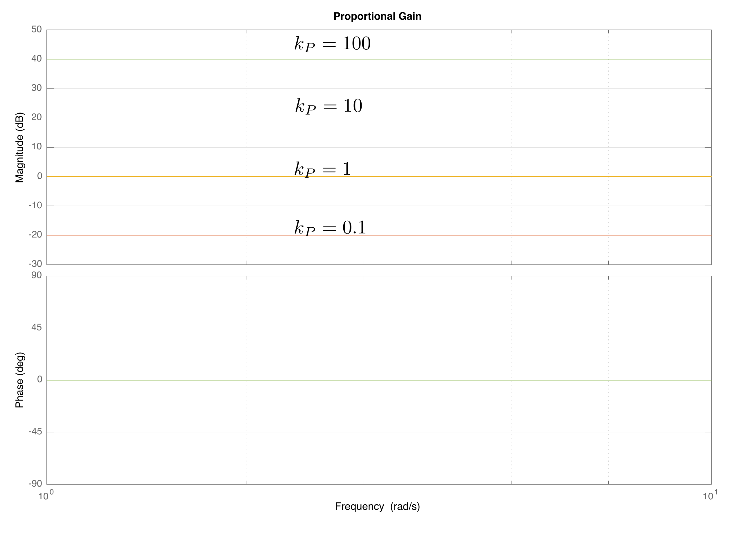
all frequencies, without affecting the phase. A Bode plot for
proportional control is shown in
Fig.18.1 for different values of
\(k_P\).
Figure 18.1. The Bode plot for proportional gain at
different values of kP. The
proportional gain adds a constant to the loop shape at all frequencies
and does not affect the phase at any frequency.
18.1.2 Building Block #2: Integral
Control
The second basic building block for loop-shaping design is
proportional-integral (PI) control where \(k_P=1\), i.e., \[C_{PI}(s) = 1+\frac{k_I}{s} =
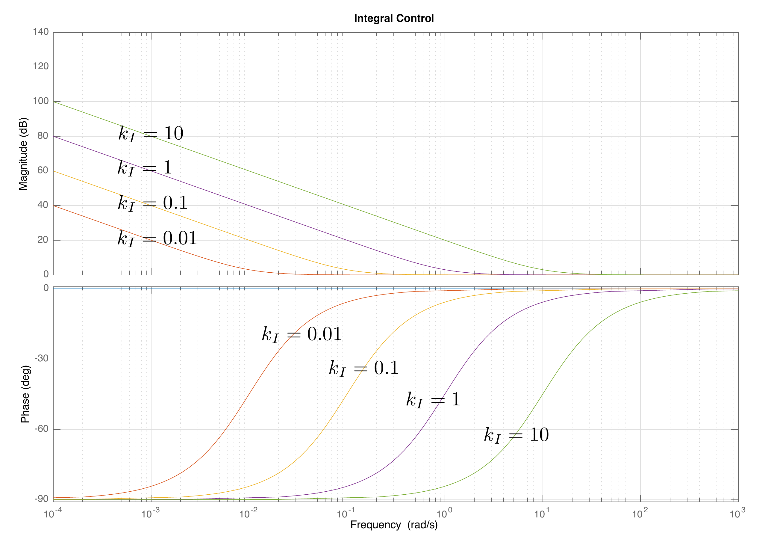
\frac{s+k_I}{s}.\] The Bode plot of \(C_{PI}\) for different values of \(k_I\) is shown in
Fig.18.2. Integral control is used
to change the system type by changing the slope of the loop gain by
\(-20\) dB/dec at low frequencies. The
Bode plot for integral control is shown in
Fig.18.2 for different values of
\(k_I\). It is clear that integral
control changes the slope for frequencies \(\omega<k_I\) while not affecting the
loop gain when \(\omega > k_I\).
Note also that integral control decreases the phase at low frequencies,
which negatively impacts stability. Therefore, integral control is
usually applied at low frequencies, where \(k_I \ll \omega_{co}\).
Figure 18.2. The Bode plot for integral control at
different values of kI. Integral
control changes the system type by decreasing the slope of the loop
shape by −20 dB/dec for frequencies
below kI,
while leaving high frequencies unaffected.
18.1.3 Building Block #3: Low-Pass
Filter
The third basic building block for loop-shaping design is a low-pass
filter where \[C_{LPF}(s) =
\frac{p}{s+p}.\] Note that the low-pass filter is constructed so
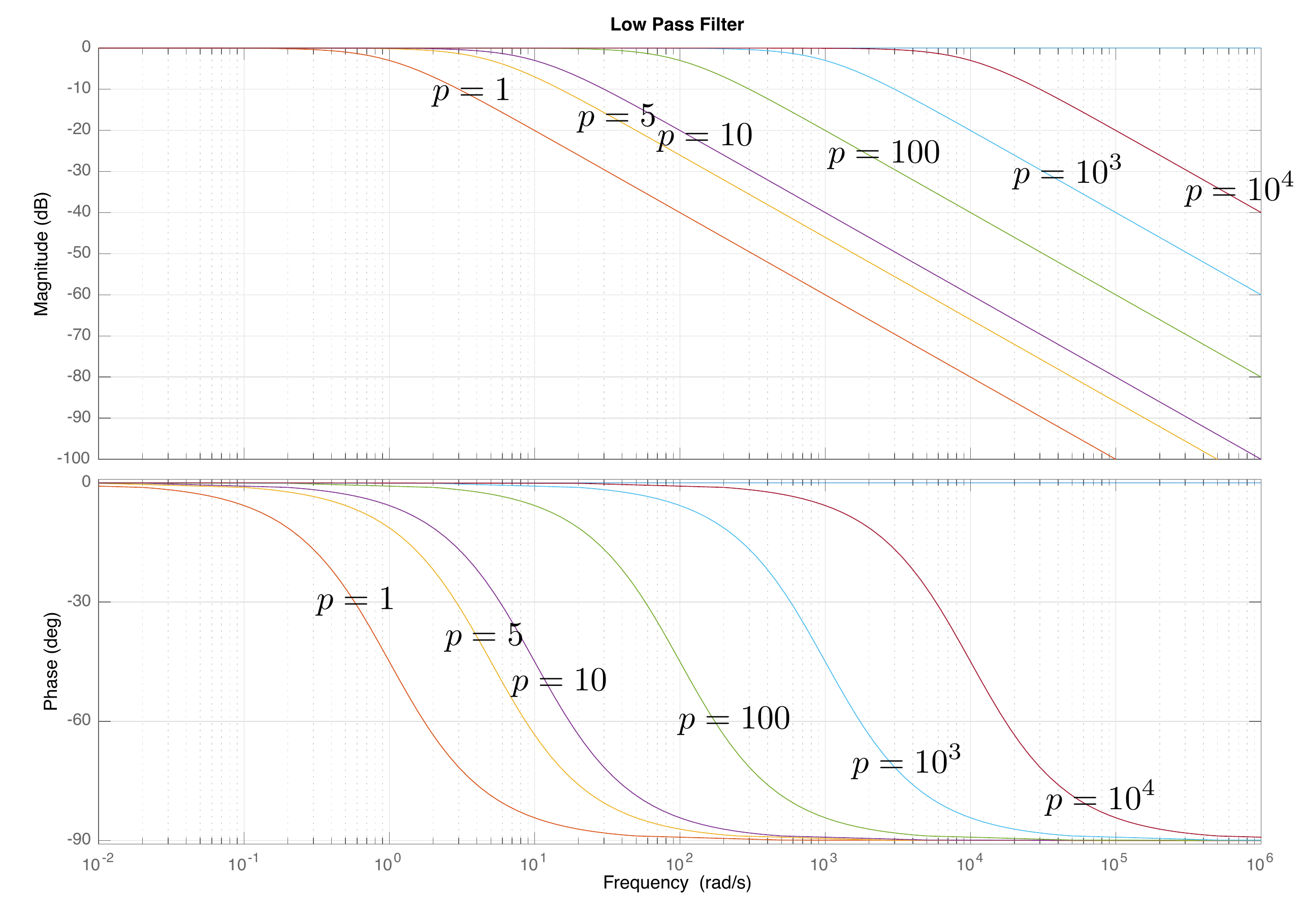
that the DC gain is one. The Bode plot for a low-pass filter is shown in
Fig.18.3 for different values of
\(p\). It is evident from
Fig.18.3 that a low-pass filter
decreases the loop gain when \(\omega>p\) while leaving the loop gain
unaffected when \(\omega<p\).
Low-pass filters are used at high frequencies to enhance noise
attenuation.
Figure 18.3. The Bode plot for a low-pass filter at
different values of the pole p. A low-pass filter decreases the
slope of the loop shape by −20 dB/dec
for frequencies above p, while
leaving low frequencies unaffected.
18.1.4 Building Block #4: Phase-Lag
Filter
The fourth basic building block for loop-shaping design is a
phase-lag filter where \[\tag{18.1}
C_{Lag}(s) = \frac{s+z}{s+p},\] where \(z>p>0\). Note that the phase-lag
filter is constructed so that \[\lim_{s\to\infty}\frac{s+z}{s+p} =
\lim_{s\to\infty}\frac{1+\frac{z}{s}}{1+\frac{p}{s}} = 1.\]
Therefore, phase-lag filters change the loop gain at low frequencies
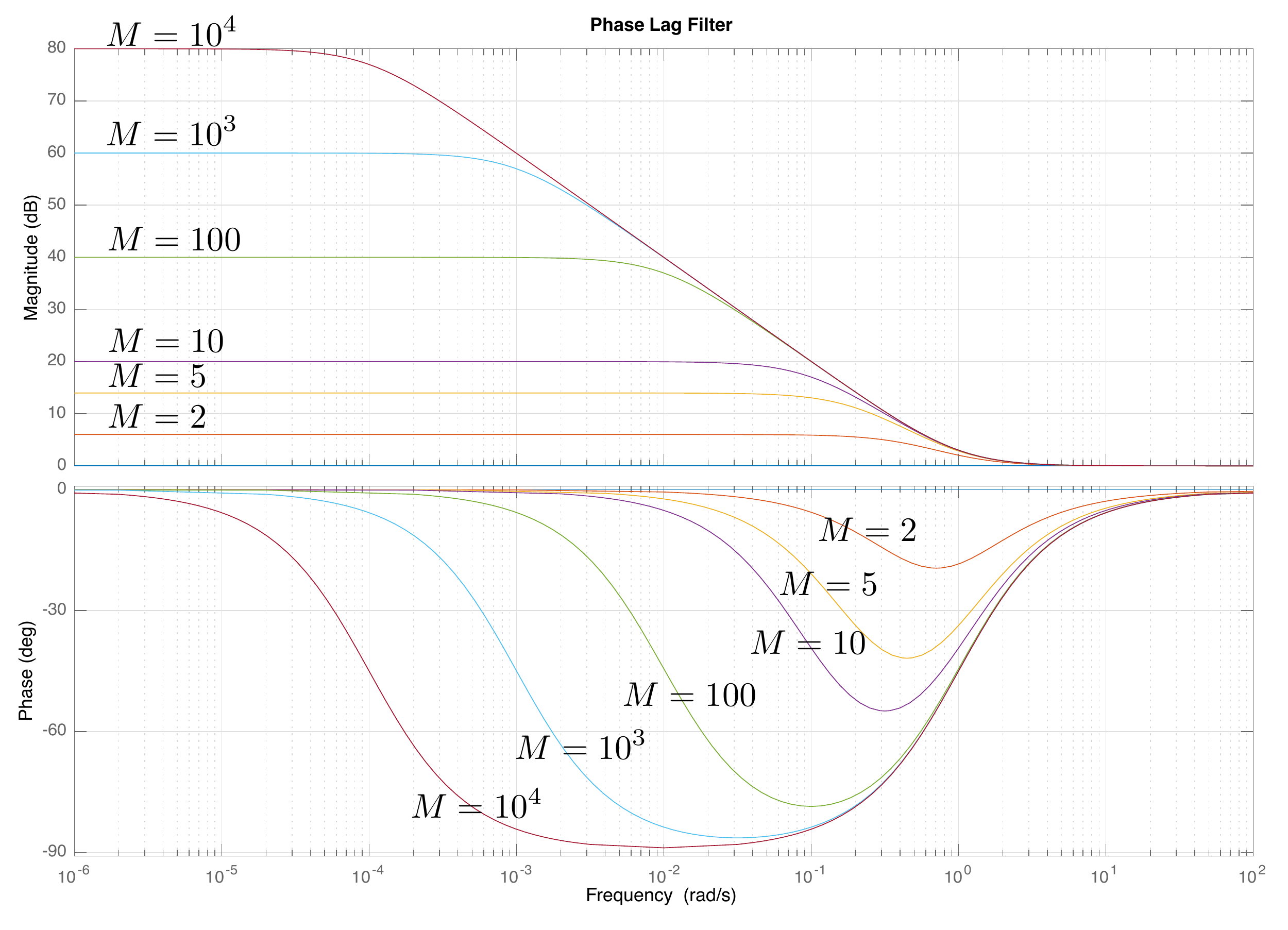
while leaving high frequencies unaffected. The Bode plot for a phase-lag
filter is shown in
Fig.18.4 when \(z=1\) and when \(p=z/M\) for different values of pole-zero
separation \(M\). Note that phase-lag
filters increase the gain at low frequencies and that the total amount
of gain is equal to the separation between the zero and the pole.
Specifically, the increased gain on the Bode plot is equal to \(20\log_{10}M\). Phase-lag filters are used
to enhance tracking performance and input/output
disturbance rejection. Unfortunately,
phase-lag filters decrease the phase between the zero and the pole and
will therefore negatively affect stability if the zero is too close to
the crossover frequency. Therefore, phase-lag filters are typically
added at low frequencies and are characterized by the zero \(z\) where the effect of the lag ends and
the pole-zero separation \(M\) which
indicates the maximum gain at low frequencies. Accordingly, the lag
filter 18.1 can be written as
\[C_{Lag}(s) =
\frac{s+z}{s+z/M}.\]
Figure 18.4. The Bode plot for a phase-lag filter when
the zero is at z = 1 and the
pole is at p = z/M, for
different values of M. A
phase-lag filter increases the loop gain at low frequencies while
leaving high frequencies unaffected.
18.1.5 Building Block #5:
phase-lead Filter
The final basic building block for loop-shaping design that we will
discuss is a phase-lead filter where \[\tag{18.2}
C_{Lead}(s) =
\left(\frac{p}{z}\right)\left(\frac{s+z}{s+p}\right),\] where
\(p>z>0\). Note that the
phase-lead filter is constructed so that \[\lim_{s\to 0}\frac{p}{z}\frac{s+z}{s+p} =
1.\] Therefore, phase-lead filters change the loop gain at high
frequencies while leaving low frequencies unaffected. The Bode plot for
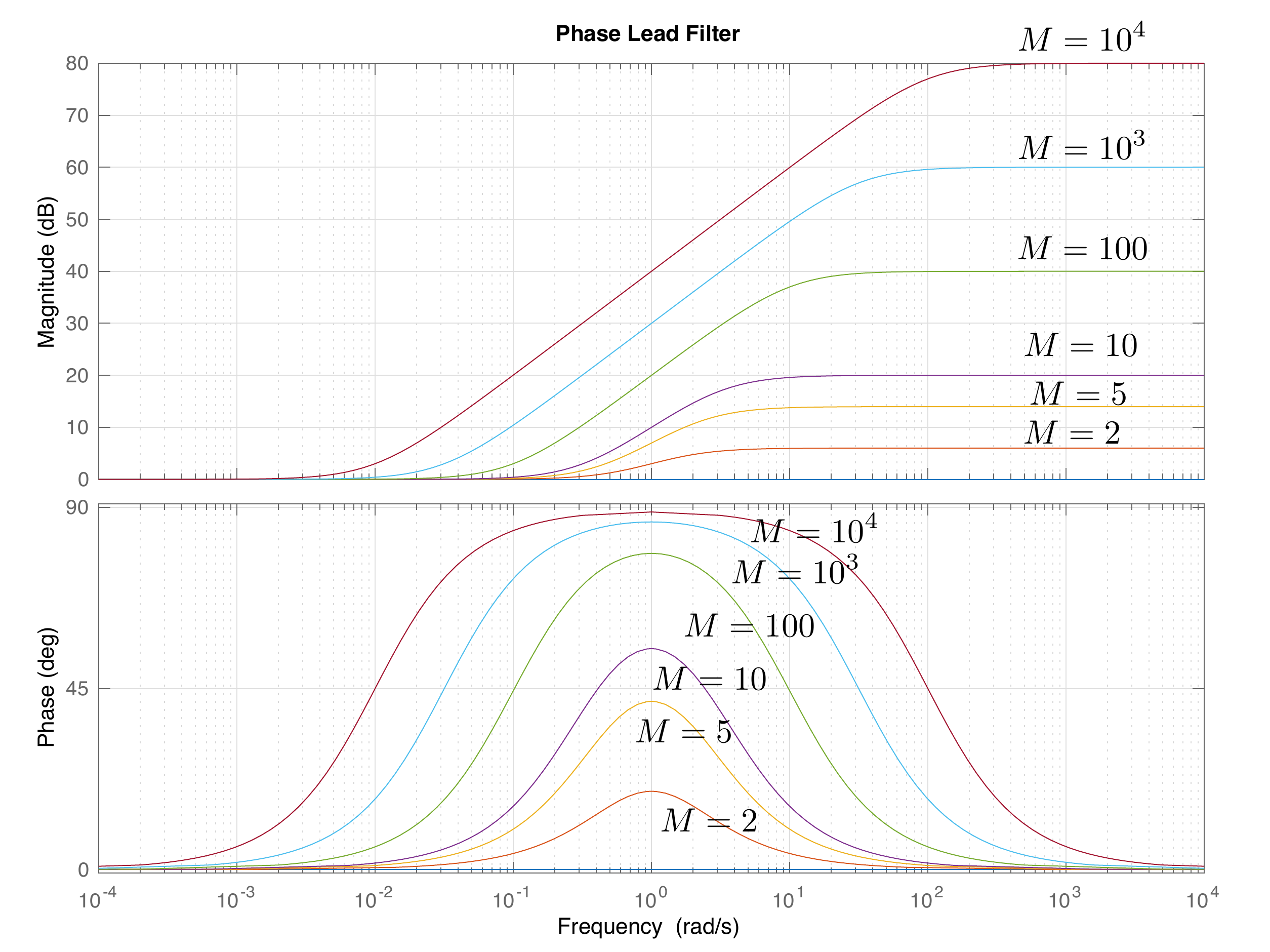
a phase-lead filter is shown in
Fig.18.5 when \(z=1\) and when \(p=Mz\) for different values of pole-zero
separation \(M\). Note that phase-lead
filters increase the phase for frequencies between the zero and the
pole. It can be shown that the peak of the phase plot shown in
Fig.18.5 is at \[\omega_{Lead} = \sqrt{zp}\] which is the
midpoint between \(z\) and \(p\) on the Bode plot. It can also be shown
that the increase in phase at \(\omega_{Lead}\) is \[\phi_{Lead} =
\tan^{-1}\sqrt{\frac{p}{z}}-\tan^{-1}\sqrt{\frac{z}{p}}.\]
Phase-lead filters are used to increase the phase margin and thereby
enhance the stability and robustness of the system. Typically, \(\omega_{Lead}\) is selected to be the
crossover frequency \(\omega_{co}\) to
obtain the maximum benefit to the phase margin. Unfortunately,
phase-lead filters also increase the loop gain at high frequencies as
shown in
Fig.18.5, which will make the
closed-loop system more sensitive to noise. Therefore, phase-lead
filters are typically accompanied by a low-pass filter at higher
frequencies. Since phase-lead filters are typically added at the
frequency giving the desired bump in phase, it is convenient to write
the transfer
function 18.2 in terms of the
center frequency \(\omega_{Lead}\) and
the lead ratio \(M\). Using the
relationship \(p=Mz\) and \(\omega_{Lead}=\sqrt{pz}\) we can write
Equation 18.2 as \[\begin{aligned}
C_{Lead}(s) &= M
\left(\frac{s+\frac{\omega_{Lead}}{\sqrt{M}}}{s+\omega_{Lead}\sqrt{M}}\right)
\\
C_{Lead}(s) &=
\frac{\frac{\sqrt{M}}{\omega_{Lead}}s+1}{\frac{1}{\omega_{Lead}\sqrt{M}}s+1}.
\end{aligned}\]
Figure 18.5. The Bode plot for a phase-lead filter
when ωLead = 1,
for different values of M. A
phase-lead filter increases the phase around ωLead.
It also increases the loop gain at high frequencies.
Chapter 18 interactive figure
Compensator building-block explorer
Choose one compensator building block. The first controls set that
block’s design parameters. The frequency marker does not change the
block; it only reads the magnitude and phase at one point on the plot.
Interactive Figure 18.I1. Move the block
parameters to see which frequency region and phase range each controller
element changes.
Transfer block
Derived pole/zero
locations
Magnitude effect
Phase effect
Best used for
Design warning
Probe readout
Check 1. Choosing a block for phase margin
If the loop shape has roughly the right
crossover frequency but the phase margin is too small, which building
block is usually the most direct choice?
Check 2.
Interpreting the lead-filter tradeoff
When you increase the phase-lead ratio M, what tradeoff should you watch
for?
Check 3. Explain a design choice
Choose one block from the explorer. In one or
two sentences, explain what frequency range it changes and what design
tradeoff it introduces.
Show
guidance
A strong response names the block, identifies
the affected frequency range, and includes the tradeoff. For example, a
low-pass filter reduces high-frequency gain for noise attenuation but
adds phase lag near the pole.
18.1.6 Simple Example 1
Given the open-loop plant \[P(s) =
\frac{1}{s+1},\] design a controller \(C(s)\) so that the closed-loop system
satisfies the following constraints:
(1) Tracks a ramp within \(\gamma_1=0.03\).
(2) Attenuate noise with frequency content above \(\omega_n=10\) rad/sec by \(\gamma_n = 0.1\).
(3) Reject input disturbances with frequency content below \(\omega_{d_{in}}=0.1\) rad/sec by \(\gamma_{d_{in}}=0.1\).
(4) Phase margin that is approximately \(60\) degrees.
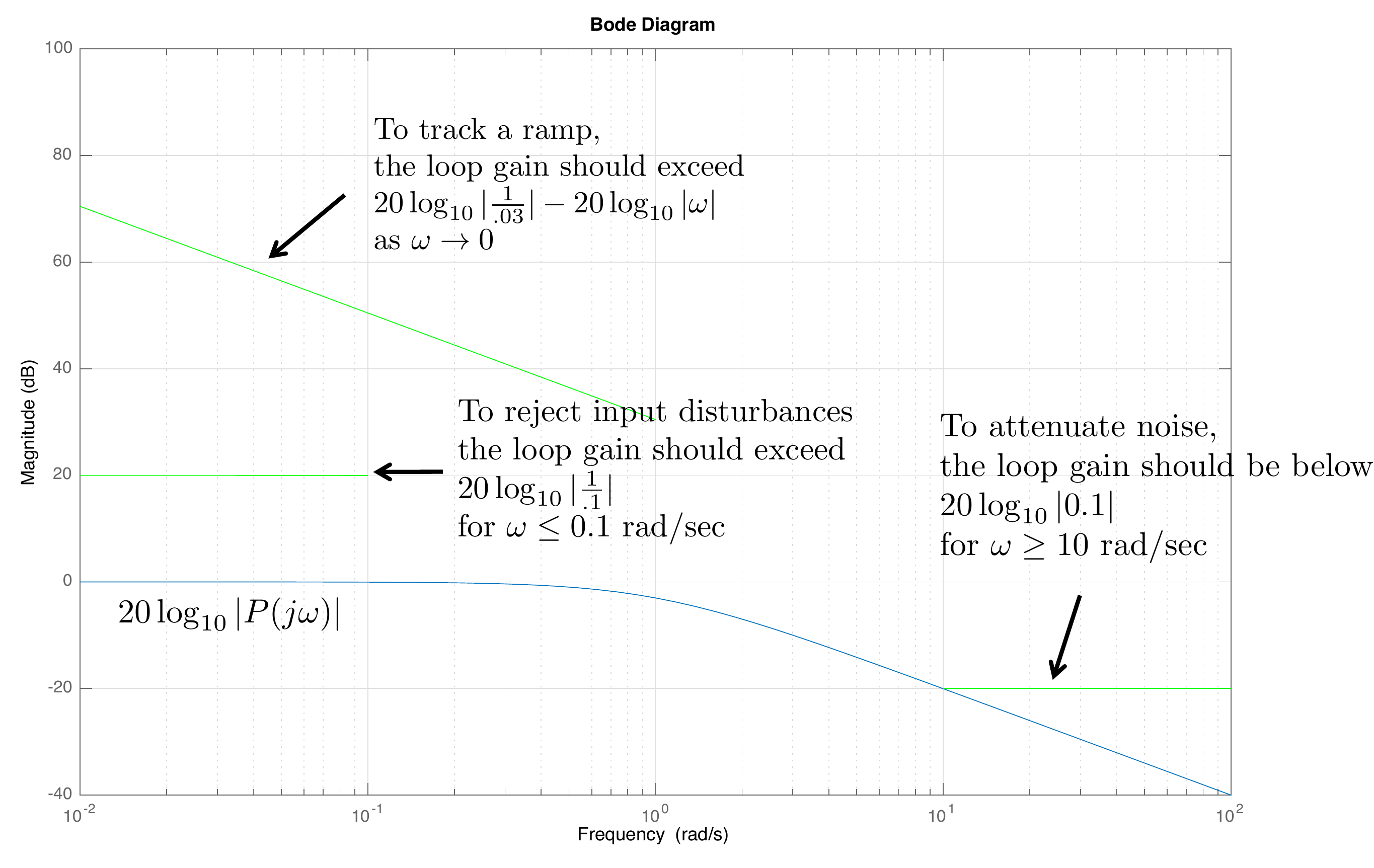
The first three design specifications can be displayed on the Bode
magnitude plot as shown in
Fig.18.6. To track a ramp
within \(\gamma_1=0.03\) requires that
the loop gain be above \[B_1 =
20\log_{10}\left|\frac{1}{0.03}\right|-20\log_{10}\left|\omega\right|\]
as \(\omega\to 0\). Therefore, to
satisfy this specification, we need to find \(C\) so that the Bode plot for \(PC\) rises above the green line on the top
left of
Fig.18.6.
To attenuate noise with frequency content above \(\omega_n=10\) rad/sec by \(\gamma_n = 0.1\), the loop gain should be
below \[B_n = 20\log_{10}\left|0.1\right| =
-20~\text{dB}\] for \(\omega>10\) rad/sec. Therefore, we need
to design \(C\) so that the Bode plot
for \(PC\) is below the green line in
the bottom right of
Fig.18.6.
To reject input disturbances with frequency content below \(\omega_{d_{in}}=0.1\) rad/sec by \(\gamma_{d_{in}}=0.1\), requires that the
loop gain is above \[20\log_{10}\left|\frac{1}{0.1}\right| +
20\log_{10}\left|P(j\omega_{d_{in}})\right| = 20-0=20\text{~dB}\]
for \(\omega<0.1\) rad/sec. Therefore, we need
to design \(C\) so that the Bode plot
for \(PC\) is above the green line in
the left-middle of
Fig.18.6.
Figure 18.6. The Bode plot for the open-loop plant in
Example 1, together with the design specifications.
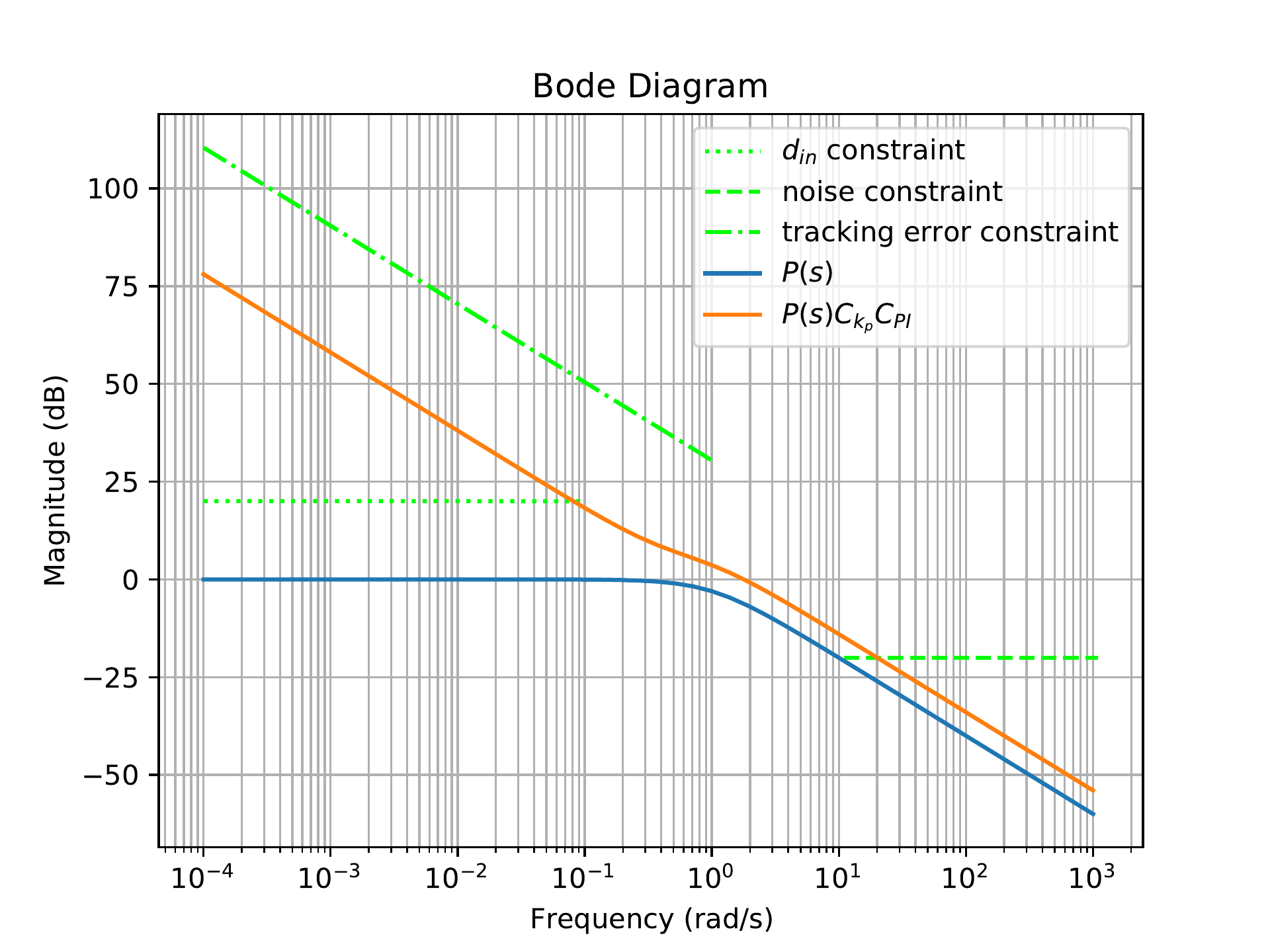
To increase the type of the system so that the slope of \(PC\) is \(-20\) dB/dec as \(\omega\to 0\), integral control can be
added.
Fig.18.7 shows the loop
gain of \(PC\) when \[C(s) = C_{P}(s)C_{PI}(s) =
\left(2\right)\left(\frac{s+0.4}{s}\right).\]
Figure 18.7. The Bode gain plot of P and PC when C includes proportional and integral
control.
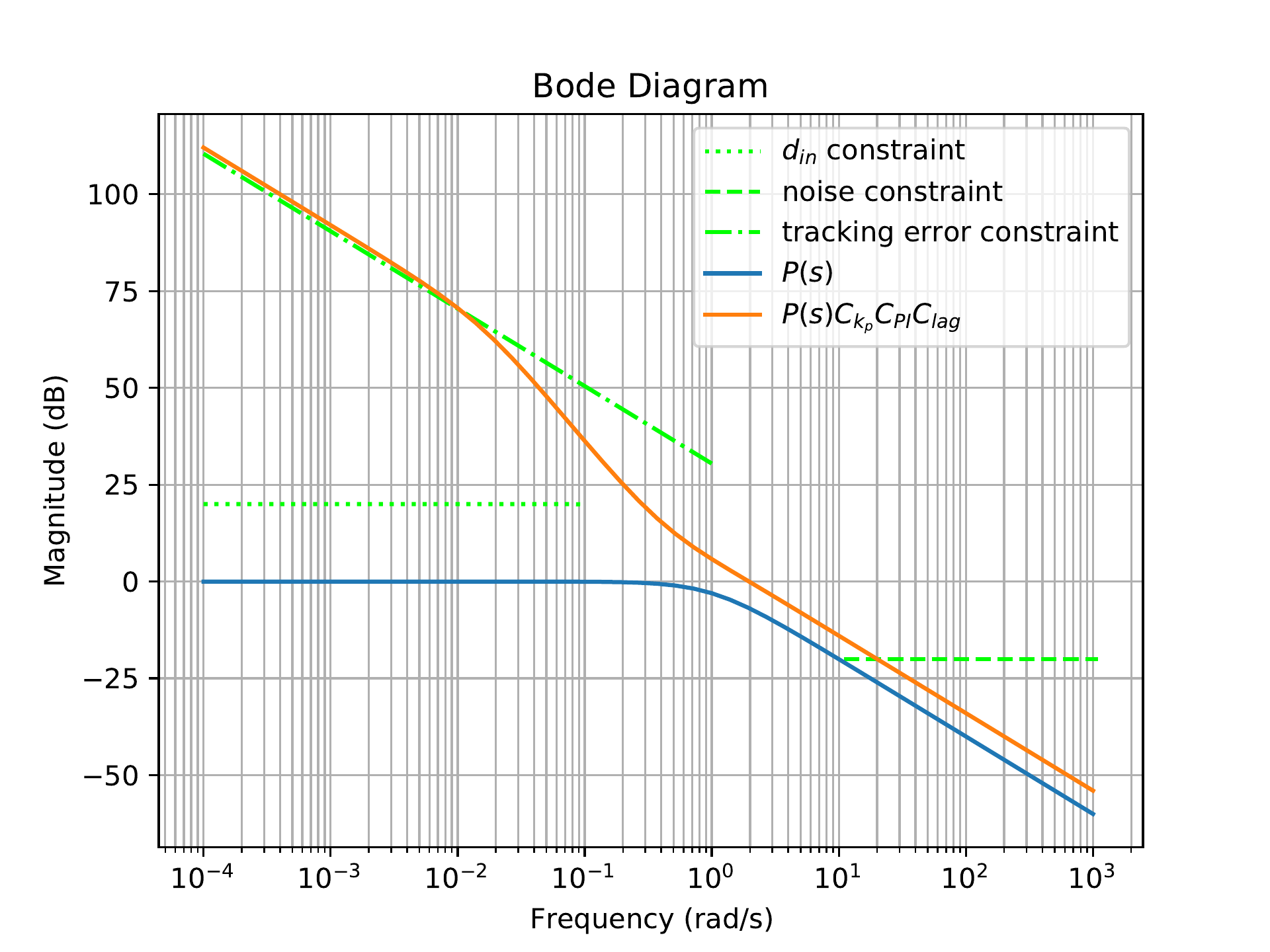
To increase the loop gain at low frequencies to get above the \(1/s\) line as \(\omega\to 0\), a phase-lag filter can be
added.
Fig.18.8 shows the loop
gain of \(PC\) when \[C(s) = C_{P}(s)C_{PI}(s)C_{Lag}(s) =
\left(2\right)\left(\frac{s+0.4}{s}\right)\left(\frac{s+0.8}{s+0.8/50}\right).\]
From
Fig.18.8 we see that the
closed-loop system will satisfy the tracking and input disturbance
specifications.
Figure 18.8. The Bode gain plot of P and PC when C includes proportional, integral,
and lag filters.
To decrease the loop gain at high frequencies to achieve the noise
attenuation specification, a low-pass filter can be added at \(p=5\).
Fig.18.9 shows the loop
gain of \(PC\) when \[\begin{aligned}
C(s) &= C_{P}(s)C_{PI}(s)C_{Lag}(s)C_{LPF}(s) \\
&=
\left(2\right)\left(\frac{s+0.4}{s}\right)\left(\frac{s+0.8}{s+0.8/50}\right)\left(\frac{5}{s+5}\right).
\end{aligned}\] The phase margin for this design is \(PM=63\) degrees and so all of the design
specifications are satisfied, as shown in
Fig.18.9.
Figure 18.9. The Bode gain plot of P and PC when C includes proportional, integral,
lag, and low-pass filters.
Chapter 18 interactive figure
Build the loop shape one compensator at a time
Step through the same loop-shaping sequence used in the example. Each
card adds one compensator block, compares the new loop shape against the
previous step, and shows which design requirements are satisfied.
Interactive Figure
18.I2. The dashed blue curve is the previous step and the solid blue
curve is the current loop shape. The bottom panel shows phase so the
crossover/phase-margin tradeoff stays visible.
Added block
Cumulative
controller
What changed?
Design prompt
Spec status
Stability context
Python code that implements this example is shown below.
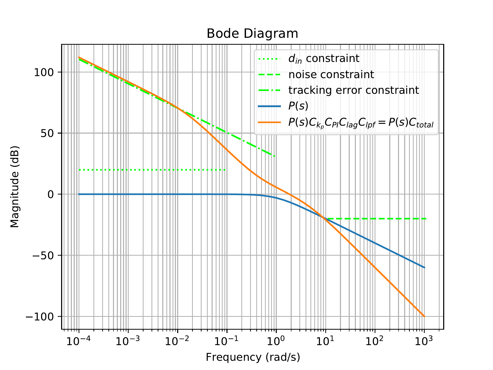
from control import*import matplotlib.pyplot as pltimport numpy as npPlant = tf([1],[1,1]) #transfer function for plant# initialize frequency response for plant onlyplt.figure()plt.grid(which='both')#################################### input disturbance specification ##################################### reject dist below this frequencyomega_din =10**-1omega = np.logspace(-4, np.log10(omega_din))Pmag, phase, _ = bode(Plant, omega, Plot=False)# amount of input disturbance in outputgamma_din =0.1mag_din =20*np.log10(1/gamma_din)*np.ones(omega.size)+20*np.log10(Pmag)plt.semilogx(omega, mag_din, color=[0, 1, 0], ls=':', label='$d_{in}$ constraint')######################## noise specification ######################### attenuate noise above this frequencyomega_n =10^1#attenuate noise by this amountgamma_n =.1omega = np.logspace(np.log10(omega_n),2+np.log10(omega_n))plt.semilogx(omega, 20*np.log10(gamma_n)*np.ones(omega.size), color=[0, 1, 0], ls='--', label='noise constraint')######################## steady state errror #########################steady state tracking of rampgamma_1 =.03omega = np.logspace(-4, 0)plt.semilogx(omega, 20*np.log10(1/gamma_1)-20*np.log10(omega), color=[0, 1, 0], ls='-.', label='tracking error constraint')# open-loop freq response for plant onlyomega = np.logspace(-4, 3)Pmag, phase, omega = bode(Plant,omega, Plot=False)Pmag_dB =20*np.log10(Pmag)plt.semilogx(omega, Pmag_dB, label='$P(s)$')################### control design ###################C =1.0#proportional controlC_kp =2.0#integral controlk_I =0.4C_PI = tf([1, k_I], [1, 0])#phase lagz =0.8M =50.0C_lag = tf([1, z], [1, z/M])#low-pass filterp =5C_lpf = tf([p], [1, p])#total filter:# for figure 18-7C1 = C*C_kp*C_PI# for figure 18-8C2 = C*C_kp*C_PI*C_lag# for figure 18-9C3 = C*C_kp*C_PI*C_lag*C_lpf# open-loop freq response of the controller + plantomega = np.logspace(-4, 3)PC_mag, phase, _ = bode(Plant*C3, omega, Plot=False)plt.semilogx(omega, 20*np.log10(PC_mag), label='$P(s)C_{k_p}C_{PI}C_{lag}C_{lpf}= P(s)C(s)$')plt.title('Bode Diagram')plt.xlabel('Frequency (rad/s)')plt.ylabel('Magnitude (dB)')plt.legend()plt.show()
18.1.7 Controller
Implementation
The loop-shaping
design procedure produces a controller \(C(s)\) that will have multiple elements,
including integrators, lead and lag filters, and low-pass filters. Each
of these elements is straightforward to implement using analog circuits.
However, if the controller is to be implemented on digital hardware
using computer code, what is the best way to proceed? While there are
many possibilities, one option that is straightforward to implement and
fits well with the previous chapters is to implement the controller
using state-space equations. The controller \[U(s) = C(s) E(s)\] is first converted to
continuous time state-space equations using, for example, control
canonical form, to produce the
equations \begin{align}
\dot{z}_C &= A_{C}z_C + B_{C}e \tag{18.3} \\
u &= C_{C}z_C + D_{C}e \tag{18.4}
\end{align} where \(e(t)=r(t)-y(t)\) is the input to the
state-space equations, and the control signal \(u(t)\) is the output. In the example of the
previous section we get \[C(s) = \frac{10 s^2
+ 12 s + 3.2}{s^3 + 5.016 s^2 + 0.08 s}.\] Therefore, using
controller canonical form, the controller implementation is \[\begin{aligned}
\dot{z}_C &= \begin{pmatrix} -5.016 & -0.08 & 0 \\ 1 & 0
& 0 \\ 0 & 1 & 0\end{pmatrix} z_C +\begin{pmatrix} 1 \\ 0 \\
0 \end{pmatrix}e \\
u &= \begin{pmatrix} 10 & 12 & 3.2 \end{pmatrix}z_C.
\end{aligned}\] In Python, the command to find the state-space
equations from the controller transfer function ‘C’ is given below:
The controller is then implemented by integrating the differential
equations between sample times. If \(T_s\) is the sample time, and \(N=10\) Euler steps are used between each
sample, then Python code that implements the controller is shown
below:
# assuming that self.z_C (the controller state) has been# initialized elsewhere and that the controller ss equations# are available in the Python classdef u = updateController(self, r, y):# calc error signal error = r - y# Euler integration steps per control calculation N =10# integrate differential equation for controllerfor i inrange(N):self.z_C =self.z_C + Ts / N * (self.A_C *self.z_C +self.B_C * error) u =self.C_C *self.z_C +self.D_C * errorreturn u
The inputs to the controller are the reference signal \(r\), the output \(y\), and the current time \(t\). The error signal is computed on
Line 5. The control
dynamics 18.3
are integrated using \(N\) Euler steps
in Lines 11–13, and the control output equation is computed in
Line 14.
18.1.8 Prefilter Design
There are applications where it is very difficult to meet the design
specifications at both low and high frequencies and still achieve a
phase margin that is close to \(60\) degrees. If for example, the phase
margin is close to \(45\) degrees, then
there will be a peak in the closed-loop Bode plot. As shown in
Fig.17.7, the peak in the
closed-loop Bode plot produces overshoot and ringing in the closed-loop
step response. One method for reducing the overshoot in the closed-loop
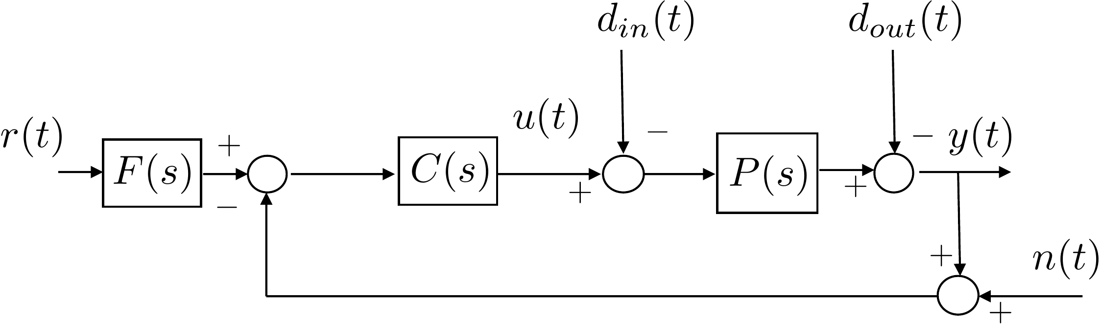
step response is to add a prefilter \(F(s)\) as shown in
Fig.18.10.
Figure 18.10. The closed-loop system with a prefilter
F(s) on the reference
command r.
The role of the prefilter \(F(s)\)
is to attenuate frequencies in \(r(t)\)
that resonate with the closed-loop system and produce the overshoot.
From a Bode plot perspective, the goal of the prefilter is to flatten
the closed-loop Bode plot so that the peak is removed. There are several
standard forms used for the prefilter. These include a notch filter and
a low-pass filter. For simplicity, we will discuss the use of a low-pass
filter below. As explained previously, the transfer function for a
low-pass filter is given by \[\tag{18.5}
F(s) = \frac{p}{s+p},\] where the DC gain is equal to one.
Just as the controller \(C(s)\) was
implemented using state-space equations, the prefilter can also be
implemented using state-space equations. The prefilter \[R_f(s) = F(s) R(s)\] is converted to
continuous time state-space equations using, for example, control
canonical form, to produce the equations \begin{align}
\dot{z}_F &= A_Fz_F + B_F r \tag{18.6} \\
r_f &= C_Fz_F + D_F r \tag{18.7}
\end{align} where the reference \(r(t)\) is the input to the state-space
equations, and the filtered reference signal \(r_f(t)\) is the output. For the transfer
function given in
Equation 18.5 we get \[\begin{aligned}
\dot{z}_F &= -p z_F + r \\
r_f &= p z_F.
\end{aligned}\]
In Python, the command to find the state-space equations is given
below, where \(F\) is the
transfer-function object representing the prefilter:
The prefilter is then implemented by integrating the differential
equations between sample times. If \(T_s\) is the sample time, and \(N=10\) Euler steps are used between each
sample, then Python code that implements the controller plus prefilter
is given below:
# assuming that self.z_C and self.z_F have been initialized# elsewhere and that the controller AND prefilter ss equations# (e.g. A_C, B_C, C_C, D_C, A_F, B_F, etc.) are available from# the Python classdef u = updateController(self, r, y):# Euler integration steps per filter calculation N =10# integrate differential equation for controllerfor i inrange(N):# prefilter the reference commandself.z_F =self.z_F + Ts / N * (self.A_F *self.z_F +self.B_F * r) r_filtered =self.C_F *self.z_F +self.D_F * r# error signal uses filtered reference error = r_filtered - yself.z_C =self.z_C + Ts / N * (self.A_C *self.z_C +self.B_C * error) u =self.C_C *self.z_C +self.D_C * errorreturn u
17.1.8.1 Prefilter Example
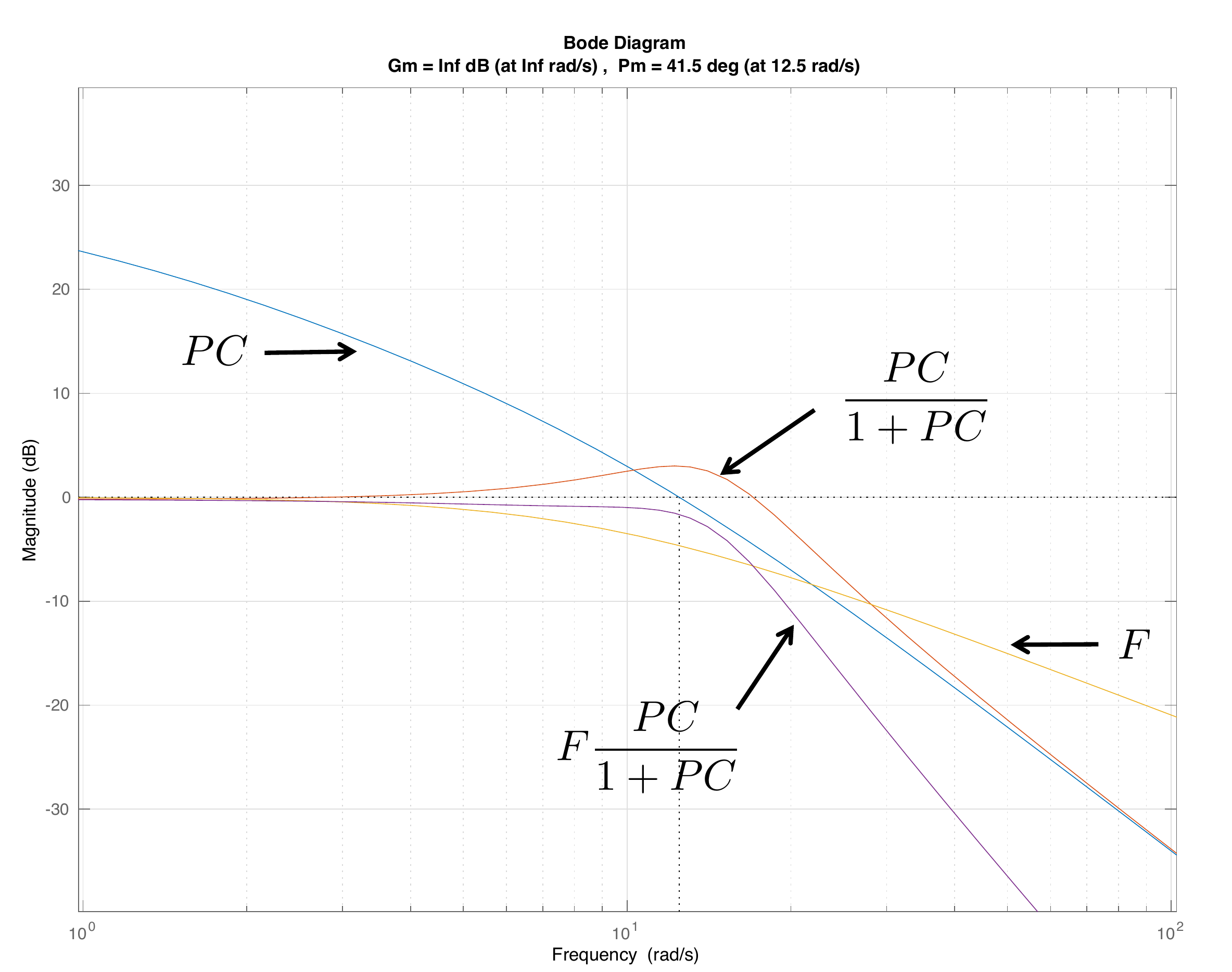
As an example, consider the open-loop system \(PC\) shown in
Fig.18.11. The phase
margin is \(PM=42.5\) degrees resulting
in a peak in the closed-loop frequency response, as shown in
Fig.18.11. The
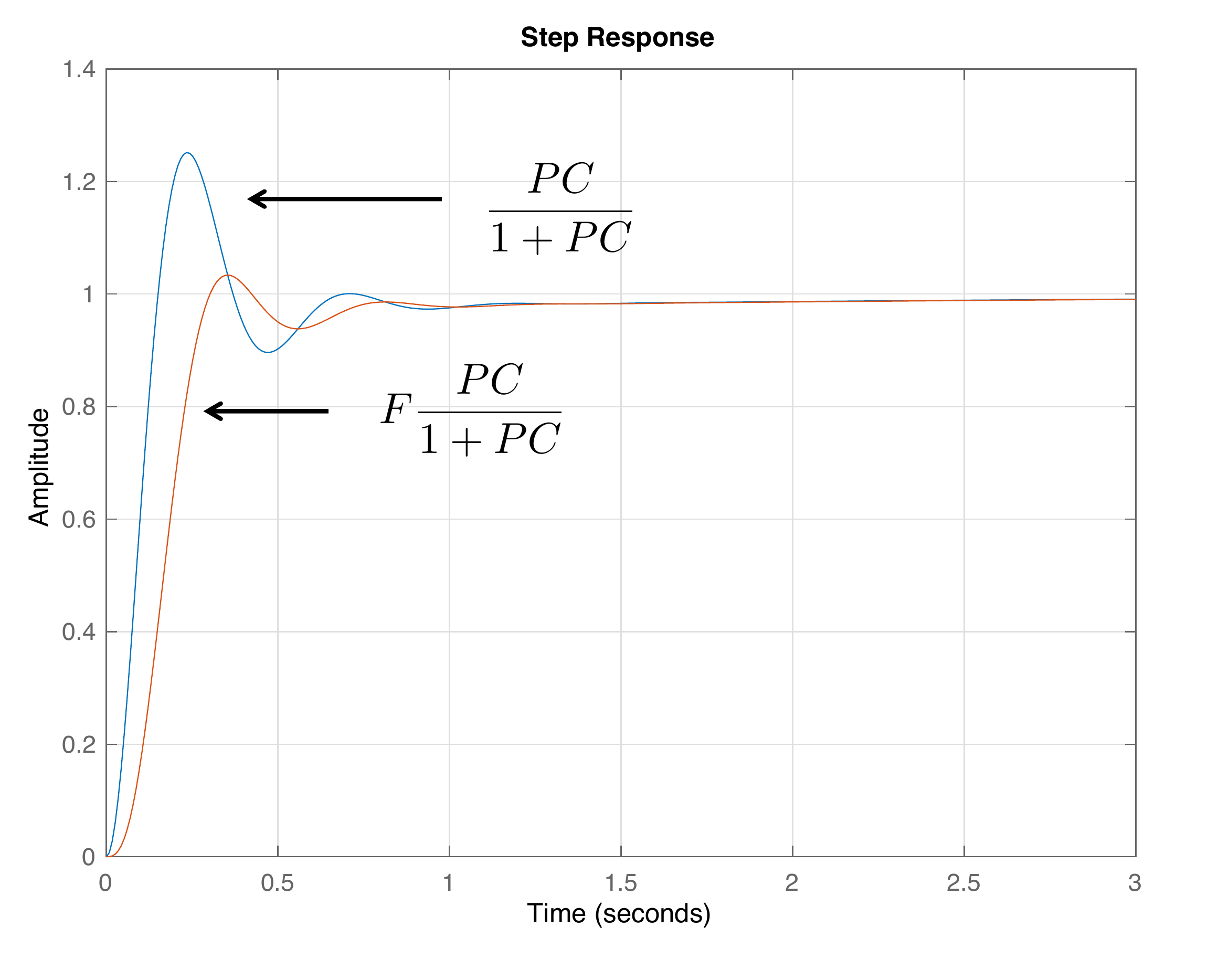
corresponding step response is shown in
Fig.18.12, where it can
be seen that there is significant ringing in the step response.
To remove the peak in the closed-loop frequency response, a prefilter
is added to the system as shown in
Fig.18.10, where the low-pass filter
pole is \(p=9\), resulting in \[F(s) = \frac{9}{s+9}.\] The Bode magnitude
of the prefilter \(F\) is shown in
Fig.18.11, as well as
the prefiltered closed-loop response \(FPC/(1+PC)\). As can be seen from
Fig.18.11, the
prefilter removes the peak in the closed-loop frequency response. The
corresponding step response is shown in
Fig.18.12, where it can
be seen that the ringing has been significantly reduced.
Figure 18.11. The loop gain for the open-loop system
PC, the closed-loop
system PC/(1 + PC),
the prefilter F, and the
closed-loop system with the prefilter FPC/(1 + PC).Figure 18.12. The step response of the closed-loop
system PC/(1 + PC)
and the closed-loop system with the prefilter FPC/(1 + PC).
Chapter 18 interactive figure
Prefilter pole and reference-response ringing
Move the prefilter pole. The frequency plot shows how the prefilter
attenuates the resonant peak, and the time plot shows the corresponding
reduction in ringing.
Interactive Figure 18.I3. A slower prefilter
removes more high-frequency command content, reducing ringing at the
cost of slower reference response.
Prefilter
Peak tendency
Step-response
tradeoff
18.1.9 Successive Loop Closure
Design
When loop shaping is
used to design an inner and outer loop controller in a successive loop
closure design, the design of the outer loop can take into account the
complete dynamics of the inner loop. This is in contrast to the design
of PID controllers in
Chapter 11 where the inner loop was
replaced with the DC gain.
Fig.18.13 shows the system architecture for
loop-shaping design. The inner and outer loop controllers are
accompanied by the prefilter \(F(s)\)
which is only on the outer loop.
Figure 18.13. The control architecture for a successive
loop closure design, with prefilter.
Step through the architecture to trace signals, close the fast inner
loop, and see how the outer-loop plant changes after the inner-loop
dynamics are collapsed into an equivalent block.
Current
task
Plant seen by
designer
Key equation
Why this step
matters
Self-check
Interactive Figure 18.I4. Trace the signals,
close the inner loop, and use the closed inner-loop dynamics as part of
the outer-loop plant.
The first step is to design the inner loop controller \(C_{in}(s)\) using the plant \(P_{in}(s)\). However, for the design of the
outer loop controller \(C_{out}(s)\),
we can use the outer loop plant in cascade with the inner closed-loop
system. Therefore, the plant for the outer loop design is given by \[P =
P_{out}\left(\frac{P_{in}C_{in}}{1+P_{in}C_{in}}\right).\]
Examples will be given in the sections below.
For this homework assignment we will use loopshaping to improve the
PID controllers developed in
HW 3.1.13. Let \(C_{pid}(s)\) be the PID controller designed
in HW 3.1.13. The final
control will be \(C(s) =
C_{pid}(s)C_{l}(s)\) where \(C_l\) is designed using loopshaping
techniques.
(a) Design \(C_l(s)\) to meet the following
objectives:
(1) Improve tracking and disturbance rejection by a factor of 10 for
reference signals and disturbances below \(0.07\) rad/sec,
(2) Improve noise attention by a factor of 10 for frequencies above \(1000\) radians/sec.
(3) Phase margin that is approximately \(PM=60\) degrees.
(b) Add zero mean Gaussian noise with standard deviation \(\sigma^2=0.01\) to the simulation developed
in HW 3.1.13.
(c) Implement the controller \(C(s)\) in
simulation using its state-space equivalent.
(d) Note that despite having a good phase margin, there is still significant
overshoot, due in part to the windup effect in the phase-lag filter.
This can be mitigated by adding a prefilter, that essentially modifies
the hard step input into the system. Add a low-pass filter for \(F(s)\) as a prefilter to flatten out the
closed-loop Bode response and implement in simulation using its
discrete-time state-space equivalent.
Design Study A guided exercise
Choose compensator building blocks
Translate each
performance shortfall into a loop-shaping compensator block.
Use the specification
regions to decide which compensator block should improve low-frequency
gain, phase margin, and high-frequency noise attenuation.
Answer: A lag compensator raises
low-frequency gain with limited effect near crossover.
Step 2.
Phase margin improvement
Show solution for Step
2
Answer: A lead compensator adds
phase near crossover and can improve phase margin.
Step 3.
High-frequency noise attenuation
Show solution for Step
3
Answer: Low-pass filtering
reduces high-frequency loop gain and attenuates sensor
noise.
Step
4. Reference-shaping block
Show solution for Step
4
Answer: A prefilter shapes the
reference command without changing the loop stability
margins.
Pseudocode
The complete solution includes loop-shaping
code. Before opening it, outline how you would build the compensator
term by term, check the Bode specifications, and compare the final step
response and control effort.
This prompt is ungraded. It is intended to
connect the compensator choices to the implementation code in the
complete solution.
Complete solution
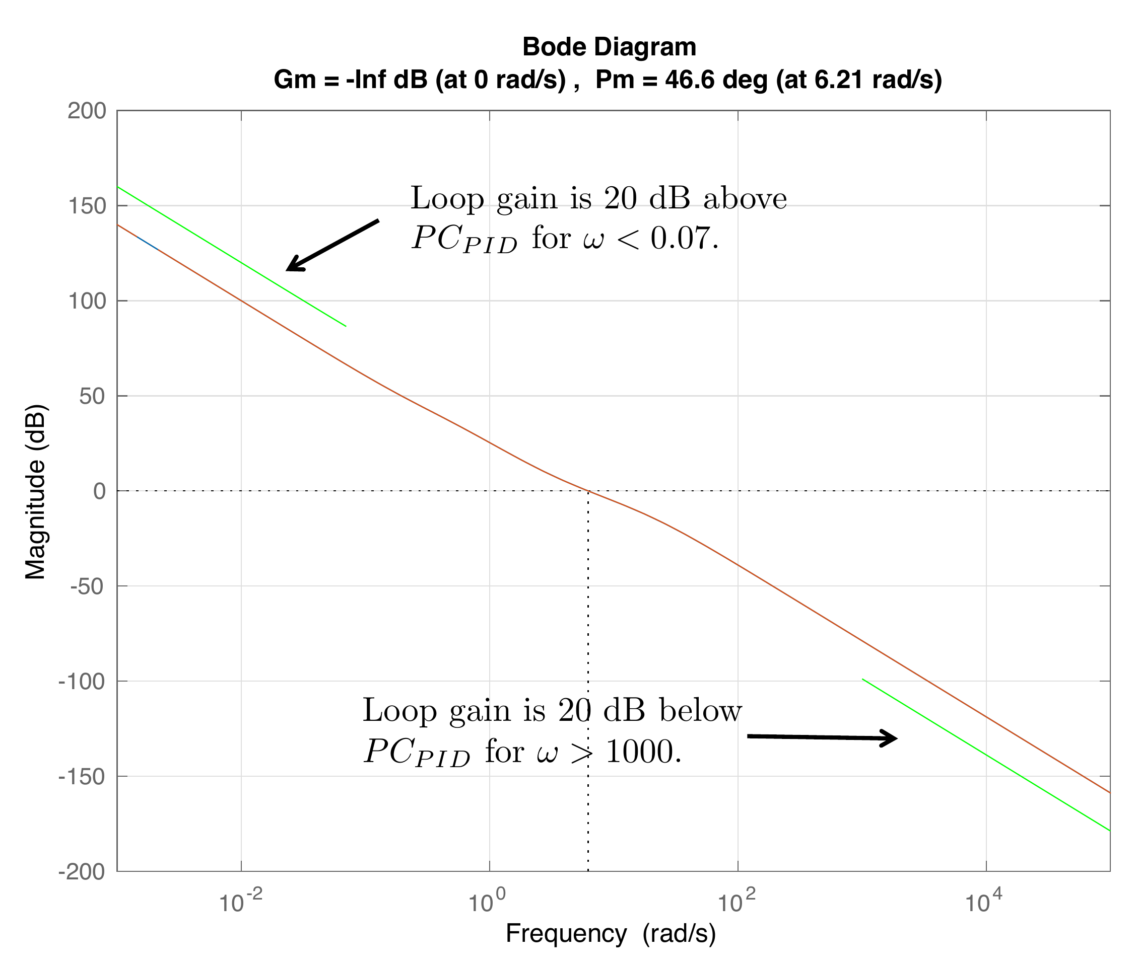
The first two design specifications can be displayed on the Bode
magnitude plot as shown in Fig.18.14. To improve
the tracking and disturbance rejection by a factor of \(10\) for reference signals and disturbances
below \(\omega_r=0.07\) rad/sec, the
loop gain must be \(20\) dB above \(P(s)C_{PID}(s)\), as shown by the green
line in the top left of Fig.18.14. To improve
noise attenuation by a factor of \(10\)
for frequencies above \(\omega_n=1000\) rad/sec, the loop gain must
be \(20\) dB below \(P(s)C_{PID}(s)\), as shown by the green
line in the bottom right of Fig.18.14.
Figure 18.14. The Bode plot for the open-loop plant in
HW 3.1.21, together with the
design specifications.
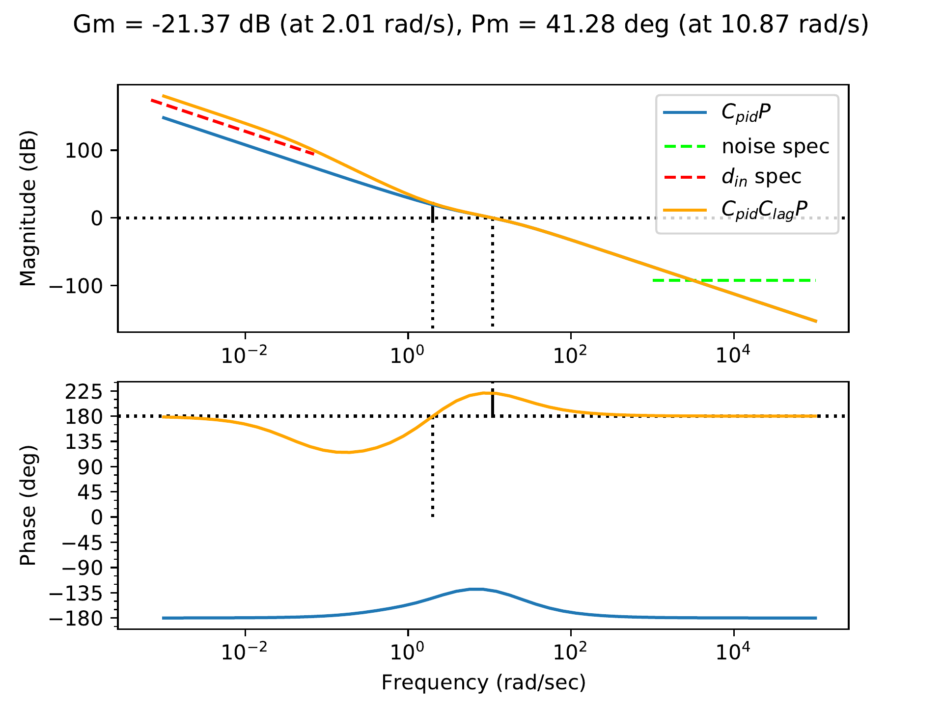
To increase the loop gain below \(\omega_r=0.07\) rad/sec, a phase-lag filter
can be added with zero at \(z=1.5\)
with a separation of \(M=40\).
Fig.18.15 shows the
loop gain of \(PC\) when \[\begin{aligned}
C(s) &= C_{PID}(s)C_{Lag}(s) \\
&= \left(\frac{0.179 s^2 + 0.554 s + 0.25}{0.05 s^2 +
s}\right)\left(\frac{s + 1.5}{s + 0.0375}\right).
\end{aligned}\] From Fig.18.15 we see that
the closed-loop system will satisfy the tracking and input disturbance
specifications.
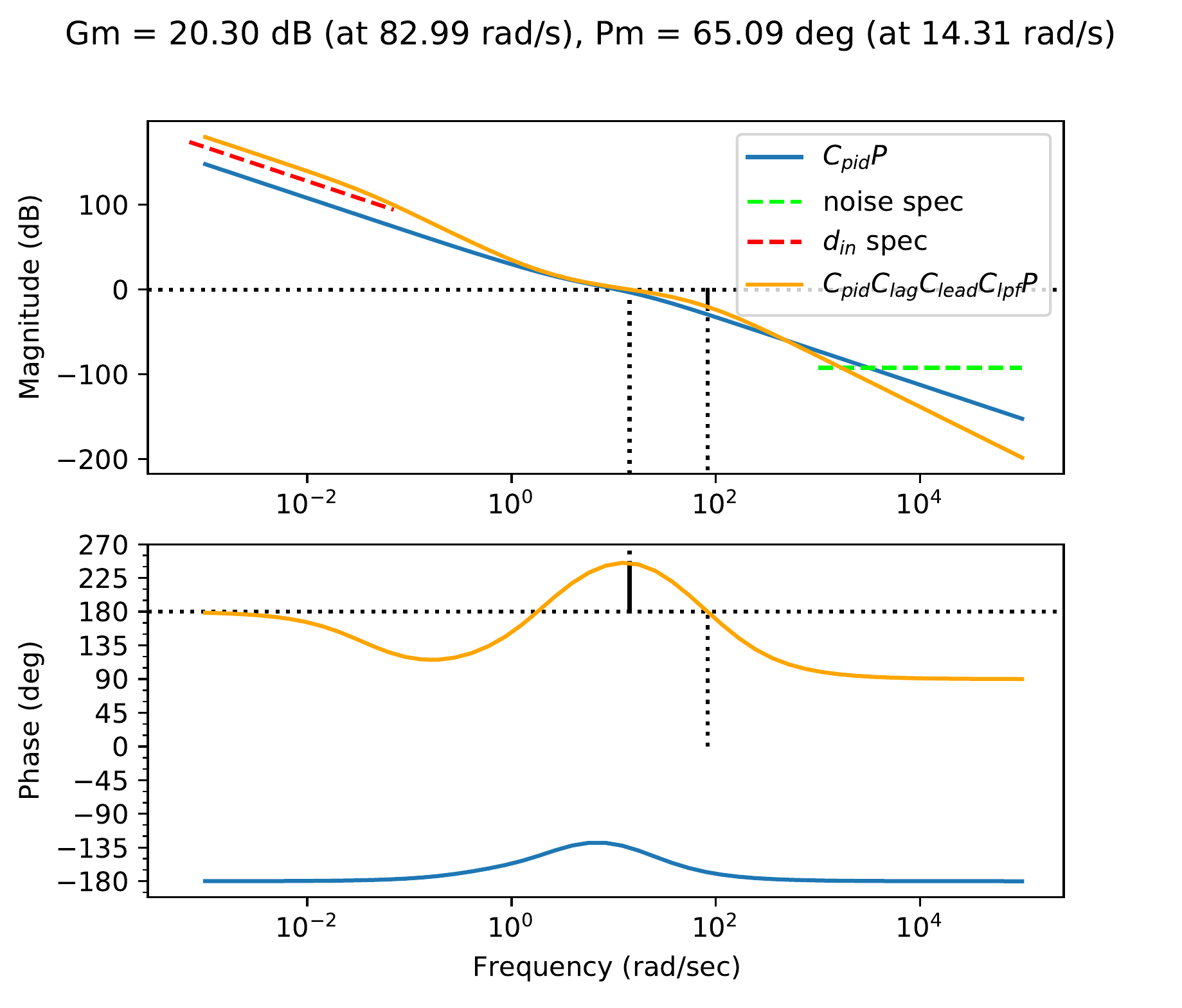
Figure 18.15. The Bode plot for HW 3.1.21 where \(C=C_{PID}C_{lag}\).
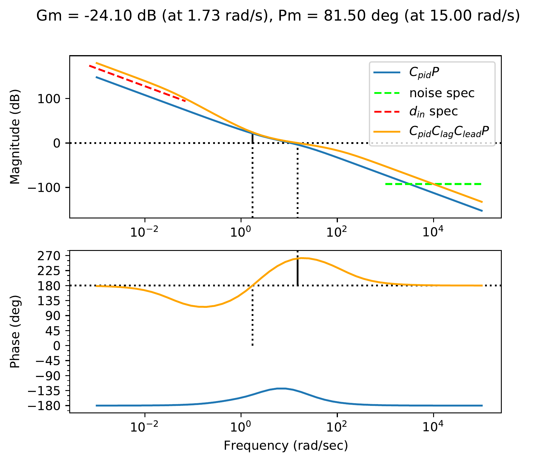
The phase margin after adding the lag filter is \(PM=41.3\) degrees. To increase the phase
margin, a phase-lead filter is added with center frequency \(\omega_c=40\) rad/sec and a separation of
\(M=10\). The center frequency for the
lead filter is selected to be above the crossover frequency so as not to
change the location of the crossover frequency, thereby keeping the
closed-loop bandwidth, and therefore the control effort, roughly the
same as with the PID controller. After adding the lead filter, the
controller is \[\begin{aligned}
C(s) &= C_{PID}(s)C_{Lag}(s)C_{Lead}(s) \\
&= \left(\frac{0.179 s^2 + 0.554 s + 0.25}{0.05 s^2 +
s}\right)\left(\frac{s + 1.5}{s + 0.0375}\right)
\left(\frac{10 s + 126.5}{s + 126.5}\right),
\end{aligned}\] and the corresponding loop gain is shown in
Fig.18.16.
Figure 18.16. The Bode plot for HW 3.1.21 where \(C=C_{PID}C_{lag}C_{lead}\).
In order to satisfy the noise attenuation specification, we start by
adding a low-pass filter at \(p=50\).
The corresponding loop gain is shown in Fig.18.17, from which
we see that the noise specification is not yet satisfied. Therefore, we
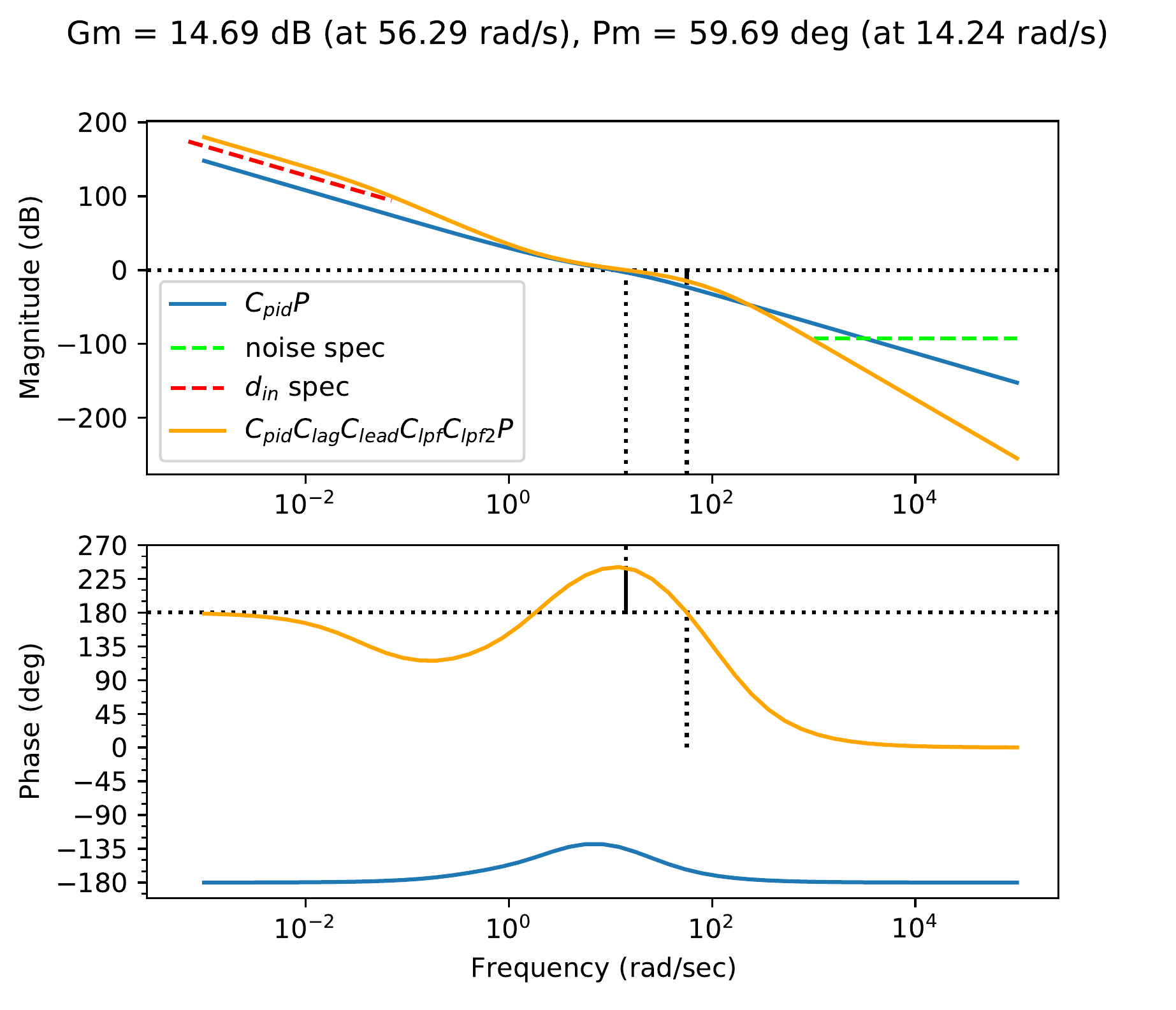
add an additional low-pass filter at \(p=150\) to obtain the loop gain in
Fig.18.18. The phase
margin is \(PM=64\) degrees. The
corresponding controller is \[\begin{aligned}
C(s) &= C_{PID}(s)C_{Lag}(s)C_{Lead}(s)C_{lpf}(s)C_{lpf2}(s) \\
&= \left(\frac{0.179 s^2 + 0.554 s + 0.25}{0.05 s^2 +
s}\right)\left(\frac{s + 1.5}{s + 0.0375}\right)\left(\frac{s + 0.7}{s +
0.07}\right)
\\ &\qquad\cdot
\left(\frac{10 s + 126.5}{s +
126.5}\right)\left(\frac{50}{s+50}\right)\left(\frac{150}{s+150}\right).
\end{aligned}\] Note that we have selected the filter values to
leave the crossover frequency the same as with the original PID
controller.
Figure 18.17. The Bode plot for HW 3.1.21 where \(C=C_{PID}C_{lag}C_{lead}C_{lpf}\).Figure 18.18. The Bode plot for HW 3.1.21 where \(C=C_{PID}C_{lag}C_{lead}C_{lpf}C_{lpf2}\).
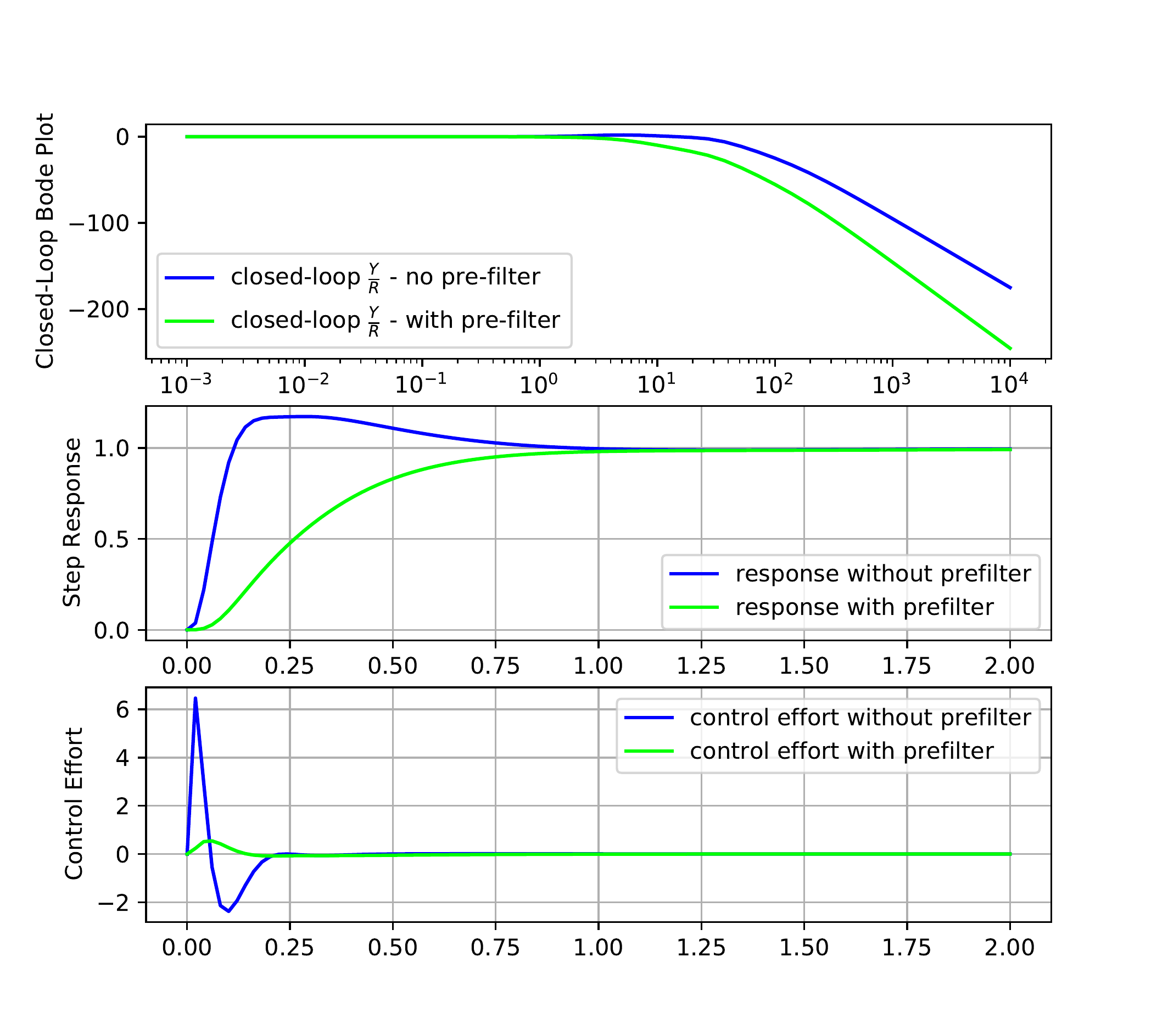
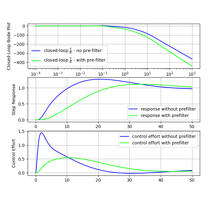
The closed-loop frequency response \(PC/(1+PC)\) and the corresponding step
response and control effort are shown by the blue lines in
Fig.18.19. The
overshoot in the step response is caused by the small amount of peaking
on the closed-loop Bode plot. The peaking can be reduced by adding a
prefilter, which in this case is a low-pass filter with pole \(p=3\). The prefiltered closed-loop
frequency response \(FPC/(1+PC)\) and
the corresponding step response and control effort are shown by the red
lines in Fig.18.19. As shown by
Fig.18.19, the
prefilter reduces the overshoot and lowers the control effort.
Figure 18.19. On the left is the closed-loop frequency
response in blue, and the prefiltered closed-loop frequency response in
red. In the middle is the associated closed-loop step response. On the
right is the associated control effort.
Python code that could be used for the design of the controller is
shown below:
# 3rd-Partyimport numpy as npimport control as cntimport matplotlib.pyplot as plt# local (controlbook)import case_studies.A_arm.params as Pfrom case_studies.A_arm.pid_controller import ArmControllerPIDimport case_studies.common.loopshaping_tools as lsuse_dB =Falseplant = cnt.tf(P.tf_num, P.tf_den)pid = ArmControllerPID()kp, ki, kd, sigma = pid.kp, pid.ki, pid.kd, pid.sigmacontroller_pid = cnt.tf([kd + kp * sigma, kp + ki * sigma, ki], [sigma, 1, 0])# original (PID) open-loop systemsys_orig_ol = cnt.series(controller_pid, plant)############################################################# design final controller by loopshaping############################################################ Because our PM starts out good enough, we will skip to adding a# low-pass filter and lag compensator to meet the low-frequency and# high-frequency requirements.C_lpf = ls.get_control_lpf(90.0)C_lag = ls.get_control_lag(z=5, M=90.0)# after checking the requirements, we need to add a lead compensator now,# along with a proportional gain and 2nd low-pass filter to meet the noise# specification.C_lead = ls.get_control_lead(omega_lead=10, M=10.0)mag, _, _ = cnt.frequency_response(sys_orig_ol, omega=[6.35])C_k = ls.get_control_proportional(1/ mag[0])C_lpf2 = ls.get_control_lpf(100.0)# this is our final controllercontroller = cnt.series( controller_pid, C_lpf, C_lag, C_lead, C_k, C_lpf2,)sys_final_ol = cnt.series(controller, plant)############################################################ add a prefilter to eliminate the overshoot###########################################################prefilter = ls.get_control_lpf(p=2.0)assert prefilter isnotNone# make type checkers happyif__name__=="__main__": _, axes = ls.plot_loopshape_stages( plant, [ ("add PID", controller_pid), ("add low-pass filter", C_lpf), ("add lag", C_lag), ("add lead", C_lead), ("set crossover gain", C_k), ("add second low-pass filter", C_lpf2), ],"Chapter 18 Loop Shaping: Single Link Arm", use_dB, omega_limits=(1e-3, 1e5), ) ax_mag = axes[0] ls.print_margins(sys_orig_ol, "Original (C_pid) Open-Loop", use_dB) ls.print_margins(sys_final_ol, "Final (C_final) Open-Loop", use_dB)# ----------- noise specification -------- omega_n =1000 improvement_factor =10.0 mag, _, _ = cnt.frequency_response(sys_orig_ol, omega=[omega_n]) gamma_n = mag[0] / improvement_factor ls.draw_noise_spec(ax_mag, gamma_n, omega_n, use_dB)# ----------- general tracking specification -------- omega_d =0.07 improvement_factor =10.0 gamma_d =1/ improvement_factor ls.draw_input_disturbance_spec(ax_mag, gamma_d, omega_d, sys_orig_ol, use_dB) ax_mag.legend() plt.show()############################################# now check the closed-loop response with prefilter############################################# Closed loop transfer function from R to Y - no prefilter tf_R_to_Y_cl = cnt.feedback(sys_final_ol, 1)# Closed loop transfer function from R to Y - with prefilter tf_R_to_Y_with_F_cl = cnt.series(prefilter, tf_R_to_Y_cl)# Closed loop transfer function from R to U - no prefilter tf_R_to_U_cl = cnt.feedback(controller, plant) # type: ignore# Closed loop transfer function from R to U - with prefilter tf_R_to_U_with_F_cl = cnt.series(prefilter, tf_R_to_U_cl) cnt.bode( [tf_R_to_Y_cl, tf_R_to_Y_with_F_cl], dB=use_dB,# plot_phase=False, label=[r"Closed-Loop $\frac{Y}{R}$ - no pre-filter",r"Closed-Loop $\frac{Y}{R}$ - with pre-filter", ], title="Closed-Loop Bode Plots: Single Link Arm", ) plt.show()## Step response plots fig3, axes3 = plt.subplots(2, sharex=True) fig3.suptitle("Closed-Loop Step Responses: Single Link Arm") time = np.linspace(0, 2, 100) ax = axes3[0] _, y_out_no_F = cnt.step_response(tf_R_to_Y_cl, time) _, y_out_F = cnt.step_response(tf_R_to_Y_with_F_cl, time) ax.plot(time, y_out_no_F, label="no prefilter") ax.plot(time, y_out_F, label="with prefilter") ax.legend() ax.grid(True) ax.set_ylabel("Step Response") ax = axes3[1] _, u_out_no_F = cnt.step_response(tf_R_to_U_cl, time) _, u_out_F = cnt.step_response(tf_R_to_U_with_F_cl, time) ax.plot(time, u_out_no_F, label="no prefilter") ax.plot(time, u_out_F, label="with prefilter") ax.set_ylabel("Control Effort") ax.set_xlabel("Time (s)") ax.grid(True) plt.show()
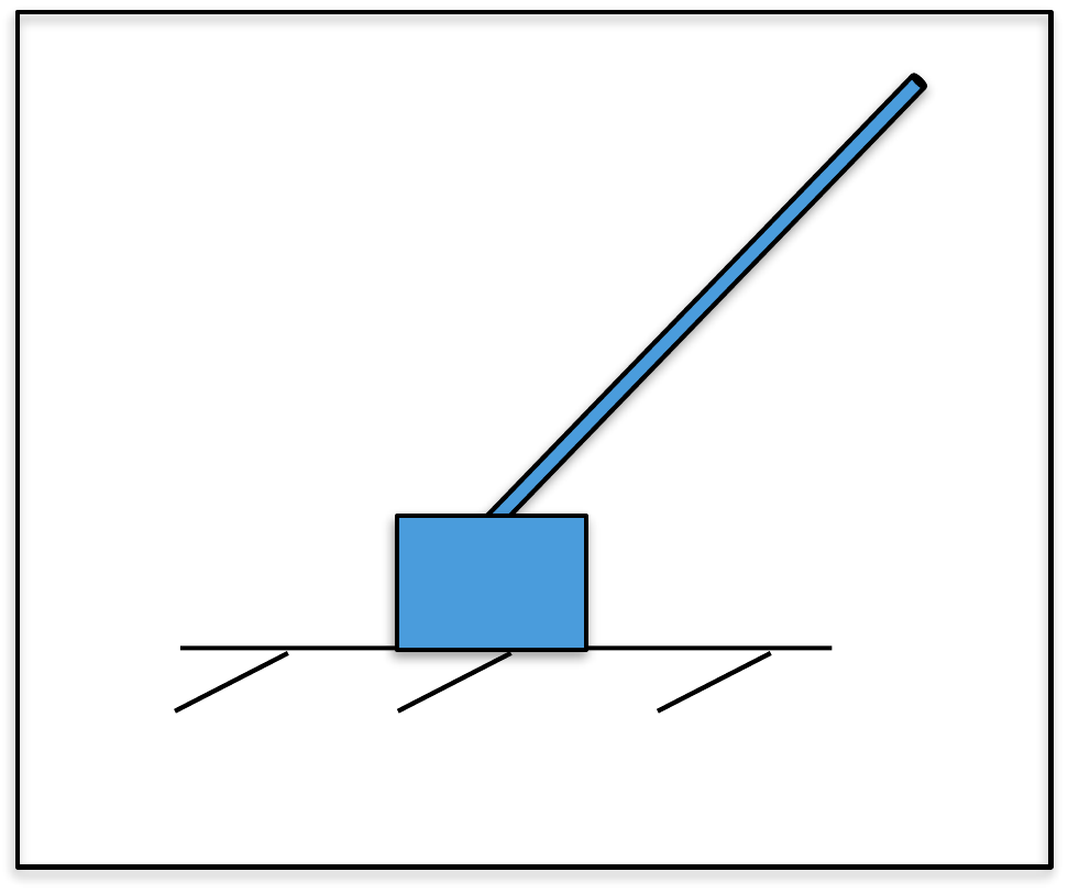
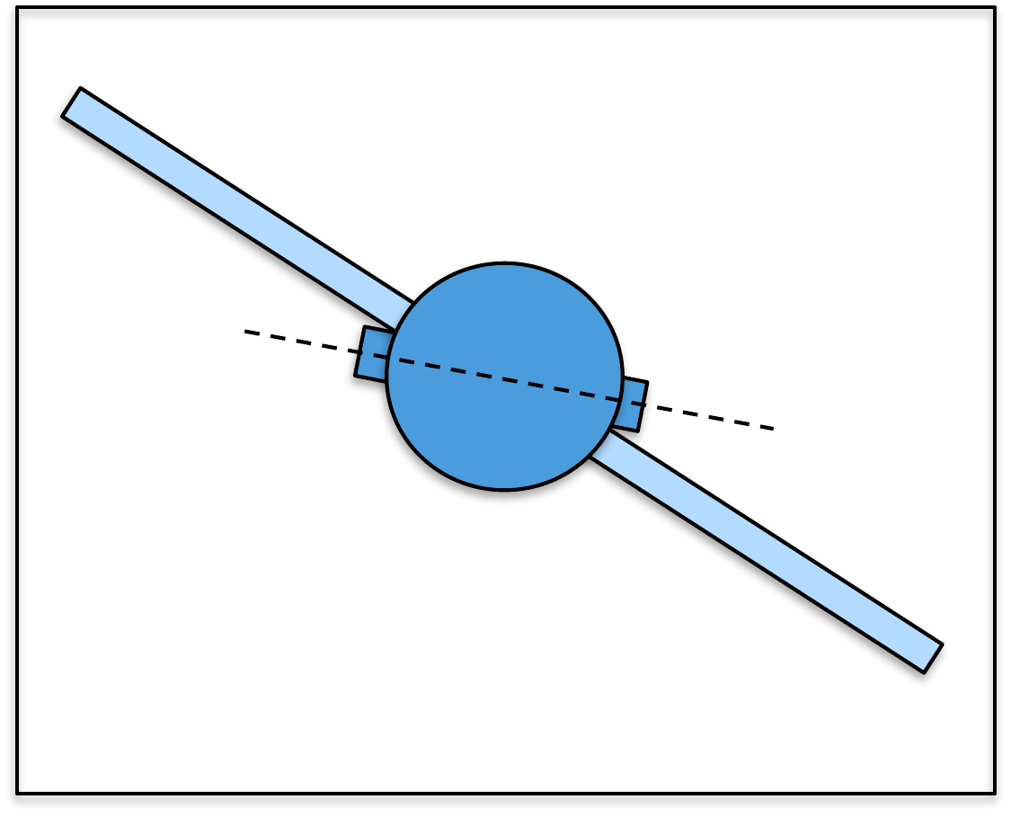
For this homework assignment we will use the loopshaping design
technique to design a successive loop closure controller for the
inverted pendulum.
First consider the inner loop, where \(P_{in}(s)\) is the transfer function of the
inner loop derived in
HW 3.2.8. Using a
proportional and phase-lead controller, design \(C_{in}(s)\) to stabilize the system with a
phase margin close to 60 deg, and to ensure that noise above \(\omega_{no}=200\) rad/s is rejected by
\(\gamma_{no}=0.1\). We want the
closed-loop bandwidth of the inner loop to be approximately 40 rad/s.
Note that since the gain on \(P_{in}(s)\) is negative, the proportional
gain will also need to be negative.
Now consider the design of the controller for the outer loop
system. The ‘plant’ for the design of the outer loop controller is \[P =
P_{out}\frac{P_{in}C_{in}}{1+P_{in}C_{in}}.\] Design the outer
loop controller \(C_{out}\) so that the
system is stable with phase margin close to \(PM=60\) degrees, and so that reference
signals with frequency below \(\omega_r=0.0032\) radians/sec are tracked
with error \(\gamma_r=0.00001\), and
noise with frequency content above \(\omega_{no}=1000\) radians/sec are rejected
with \(\gamma_{no}=0.0001\). Design the
crossover frequency so that the rise time of the system is about
2 sec.
Design
Study B guided exercise
Plan the pendulum loop-shaping
design
Choose compensator building blocks for inner and
outer loop requirements.
Start with the inner-loop plant and design
blocks that stabilize the upright pendulum while satisfying noise and
bandwidth requirements.
Step 1.
Proportional gain sign
Show
solution for Step 1
Answer: The
inner plant has negative gain, so the stabilizing proportional gain is
negative.
Step 2.
Phase-margin block
Show
solution for Step 2
Answer: Lead
compensation adds phase near crossover.
Step 3.
Noise requirement
Show
solution for Step 3
Answer: The
inner-loop design must reject noise above 200 rad/s.
Pseudocode
The complete solution includes separate
loop-shaping scripts for the inner and outer loops. Before opening it,
outline each component separately.
These prompts are ungraded. They are
intended to connect the derivation to the implementation code in the
complete solution.
Complete solution
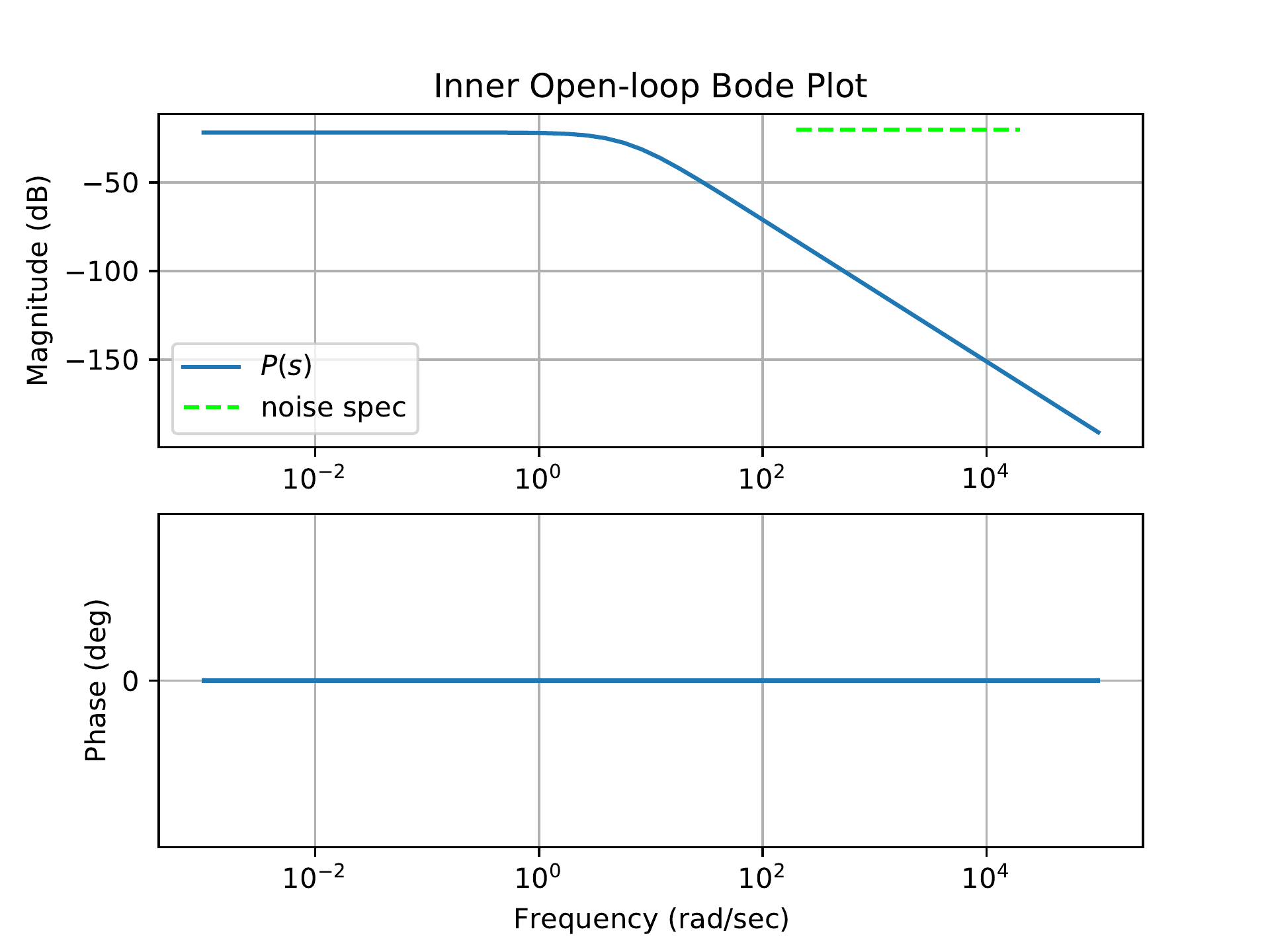
Fig.18.20 shows
the Bode plot of the plant \(P_{in}(s)\) together with the design
specification on the noise attenuation.
Figure 18.20. The Bode plot for the inner loop plant in
HW 3.2.21, together with the
design specification.
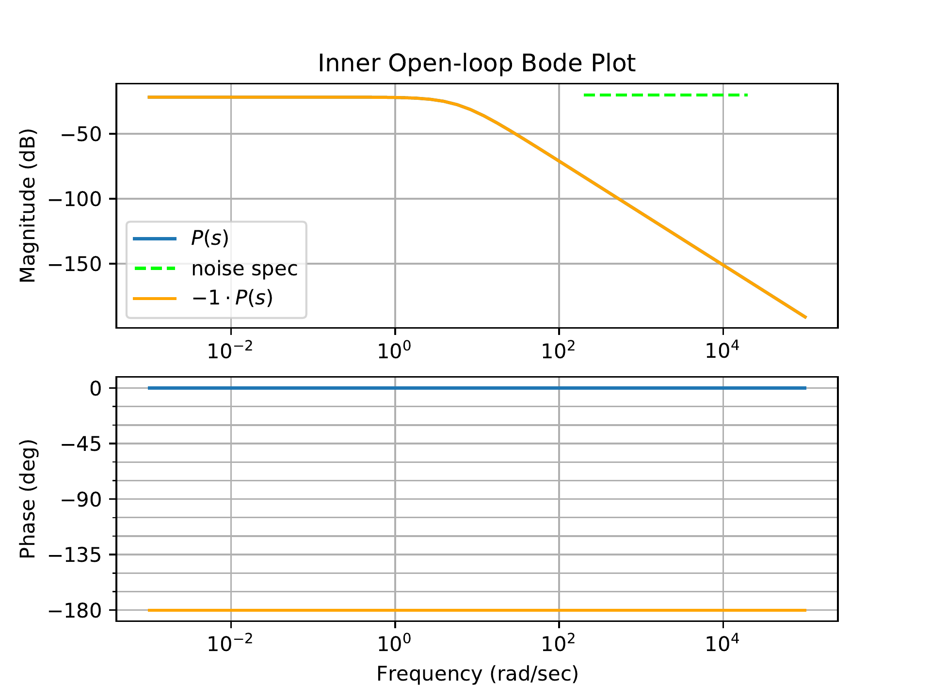
The first step is to add a negative proportional gain of 1 to account
for the negative sign in the plant transfer function.
Fig.18.21 shows
the corresponding Bode plot for a proportional gain of \(K=-1\). Once this is applied the phase of
the plant alone is \(-180\) deg over
all frequencies.
Figure 18.21. The Bode plot for the inner loop plant in
HW 3.2.21, with a gain of \(-1\) applied.
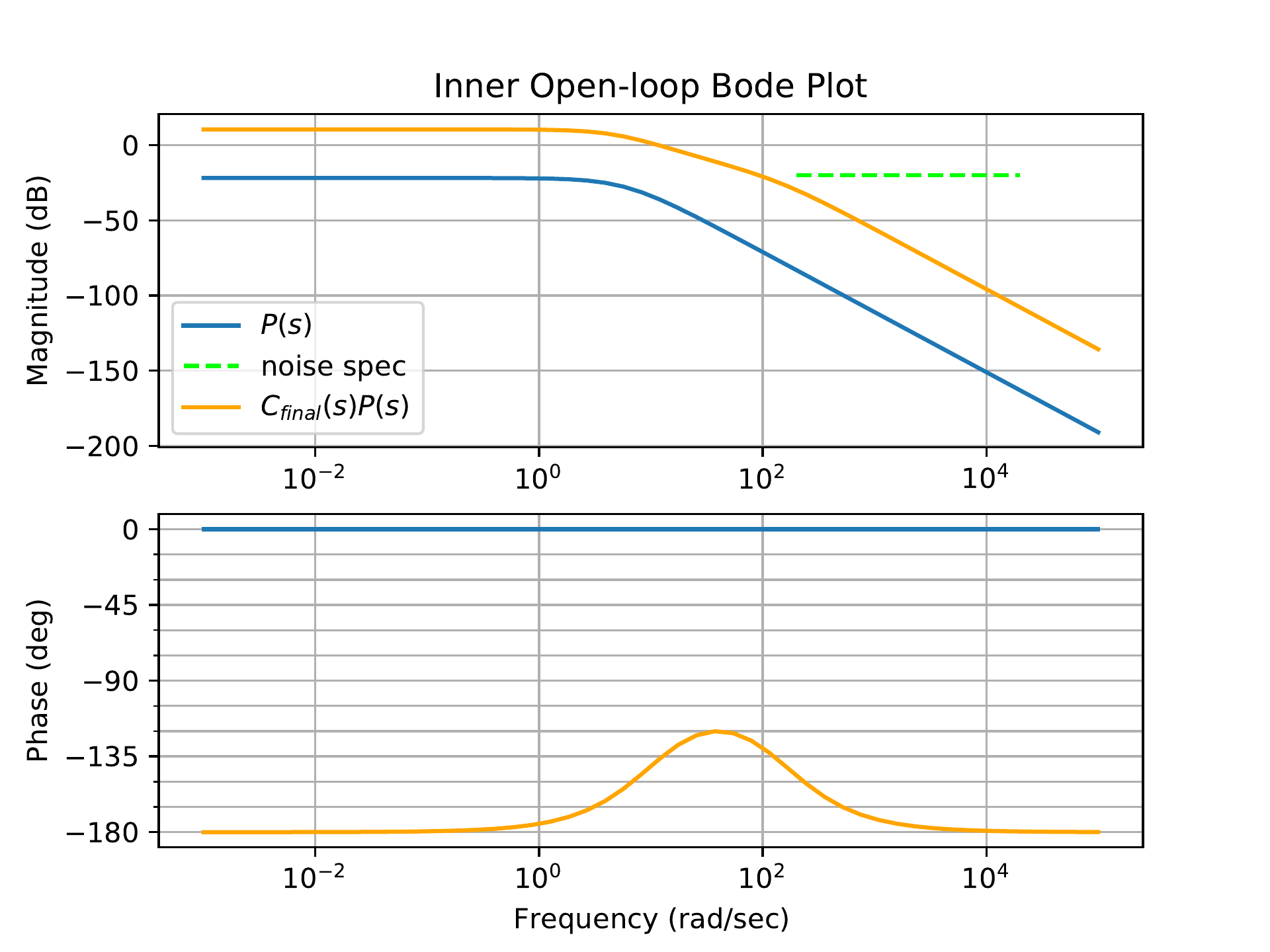
We want the bandwidth of the inner loop to be approximately 40 rad/s,
so we will set the crossover frequency to 40 rad/s. To stabilize the
system, we will add lead compensation centered at 40 rad/s with a lead
ratio of 13.9 that corresponds to the desired phase margin of 60 deg.
Fig.18.22 shows
the addition of the phase-lead filter \[C_{lead} = -155.12\left(
\frac{\frac{s}{10.72}+1}{\frac{s}{120}+1} \right),\] which has a
phase margin of \(PM=60\) degrees. The
gain 155.12 sets the crossover frequency to be 40 rad/s. The lead
compensation alone also satisfies the noise specification.
Figure 18.22. The Bode plot for the inner loop system
in HW 3.2.21, with proportional gain
and phase-lead compensation.
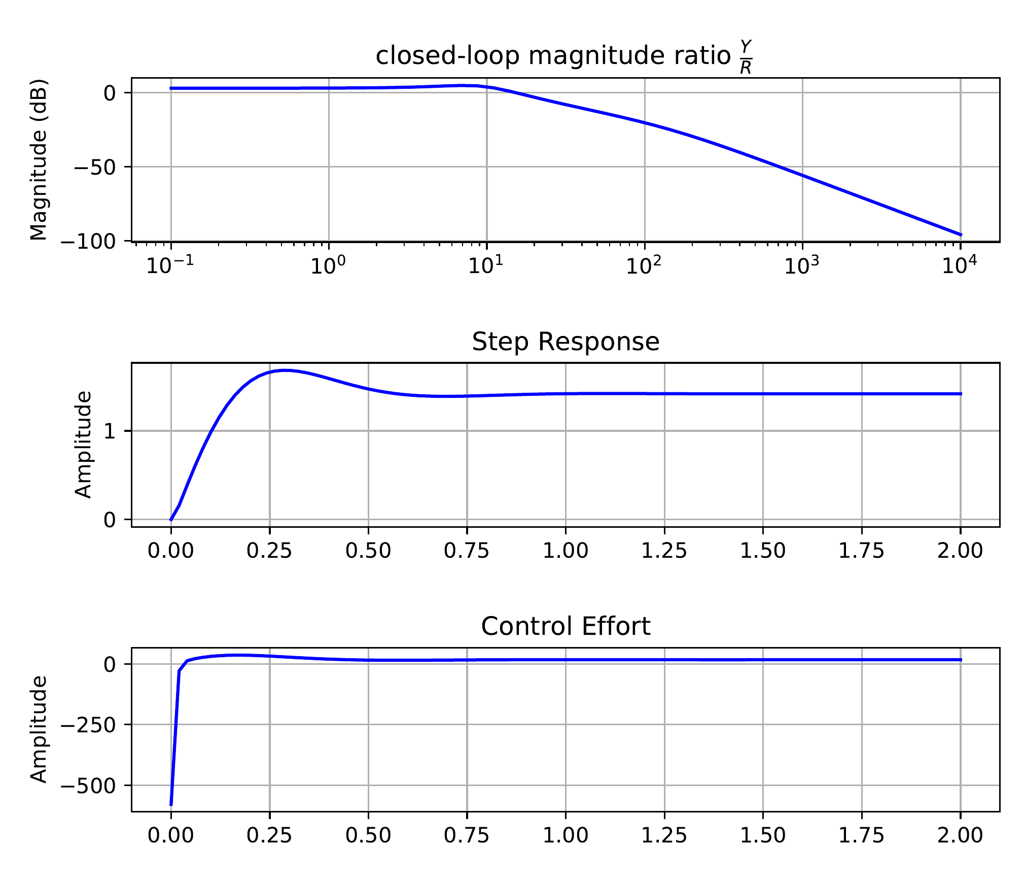
Notice that the DC gain is not equal to one. The closed-loop
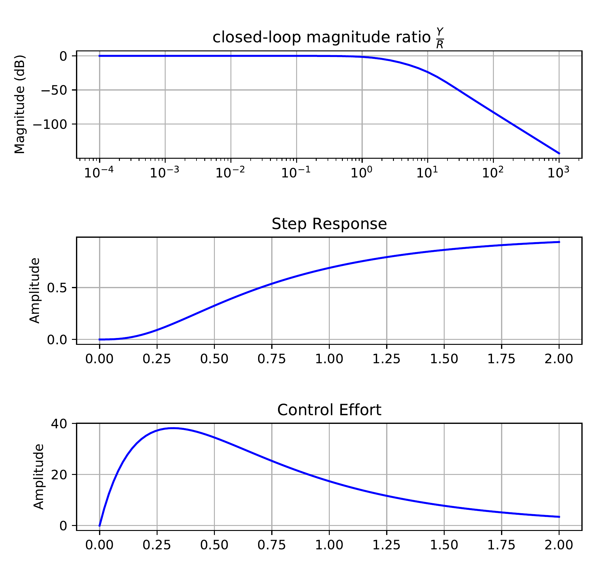
magnitude response for the inner-loop subsystem \[\frac{P_{in}C_{in}}{1+P_{in}C_{in}},\] as
well as the unit step response for the output and control signal are all
shown in Fig.18.23.
Figure 18.23. The closed-loop Bode response, the unit
step response for the output, and the unit step response for the input
of the inner loop design in HW 3.2.21.
The Python code used to design the inner loop is shown below.
# 3rd-Partyimport numpy as npimport control as cntimport matplotlib.pyplot as plt# local (controlbook)import case_studies.B_pendulum.params as Pimport case_studies.common.loopshaping_tools as lsuse_dB =Falseplant_inner = cnt.tf(P.tf_inner_num, P.tf_inner_den)plant_outer = cnt.tf(P.tf_outer_num, P.tf_outer_den)############################################################# design controllers by loopshaping############################################################ ----------- inner loop -----------C_k_inner = ls.get_control_proportional(kp=-200.0)C_lead_inner = ls.get_control_lead(omega_lead=40.0, M=15.0)controller_inner = cnt.series(C_k_inner, C_lead_inner)sys_inner_ol = cnt.series(controller_inner, plant_inner)sys_inner_cl = cnt.feedback(sys_inner_ol, 1)# ----------- outer loop -----------# update the plant to include the inner loopplant_outer = cnt.series(sys_inner_cl, plant_outer)C_k_outer = ls.get_control_proportional(kp=0.023)C_lead_outer = ls.get_control_lead(omega_lead=1.0, M=18.0)C_lag_outer = ls.get_control_lag(z=0.04, M=5.0)C_lpf_outer = ls.get_control_lpf(p=50.0)controller_outer = cnt.series( C_k_outer, C_lead_outer, C_lag_outer, C_lpf_outer,)sys_outer_ol = cnt.series(controller_outer, plant_outer)sys_outer_cl = cnt.feedback(sys_outer_ol, 1)############################################################ add a prefilter to eliminate the overshoot###########################################################prefilter = ls.get_control_lpf(p=2.0)assert prefilter isnotNone# make type checkers happyif__name__=="__main__":############################################# inner loop############################################ w_lims = (1.0, 1e3) fig, ax = ls.plot_loopshape_stages( plant_inner, [ ("add proportional gain", C_k_inner), ("add lead", C_lead_inner), ],"Chapter 18 Loop Shaping: Pendulum on a Cart - Inner Loop", use_dB, omega_limits=w_lims, ) cnt.bode( sys_inner_cl, ax=ax, dB=use_dB, omega_limits=w_lims, grid=False, label="closed-loop", ) ax_mag = ax[0] ls.print_margins(sys_inner_ol, "Open-Loop (inner)", use_dB)# ----------- noise specification -------- omega_n =200.0 gamma_n =0.1 ls.draw_noise_spec(ax_mag, gamma_n, omega_n, use_dB)# ----------- bandwidth -------- bw_desired =40.0 bw_actual = cnt.bandwidth(sys_inner_cl) ax_mag.axvline(x=bw_actual, color="black", linestyle="-", label="bandwidth") ax_mag.axvline(x=bw_desired, color="red", linestyle="-.", label="bandwidth spec") ax_mag.legend(ncol=2, loc="lower left", fontsize="small") fig.tight_layout() plt.show()############################################# outer loop############################################ w_lims = (1e-3, 1e4) fig, ax = ls.plot_loopshape_stages( plant_outer, [ ("add proportional gain", C_k_outer), ("add lead", C_lead_outer), ("add lag", C_lag_outer), ("add low-pass filter", C_lpf_outer), ],"Chapter 18 Loop Shaping: Pendulum on a Cart - Outer Loop", use_dB, omega_limits=w_lims, )# cnt.bode(# sys_outer_cl,# ax=ax,# dB=use_dB,# omega_limits=w_lims,# grid=False,# label="closed-loop",# ) ax_mag = ax[0] ls.print_margins(sys_outer_ol, "Open-Loop (outer)", use_dB)# ----------- noise specification -------- omega_n =1000.0 gamma_n =0.0001 ls.draw_noise_spec(ax_mag, gamma_n, omega_n, use_dB)# ----------- tracking specification -------- omgega_r =0.0032 gamma_r =0.00001 ls.draw_ref_tracking_spec(ax_mag, gamma_r, omgega_r, use_dB)# ----------- crossover frequency -------- tr_des =2.0 wc_des =2.2/ tr_des# ax_mag.axvline(x=bw_actual, color="black", linestyle="-", label="bandwidth") ax_mag.axvline(x=wc_des, color="red", linestyle="-.", label=r"$\omega_c$ spec") ax_mag.legend(ncol=2, loc="lower left", fontsize="small") fig.tight_layout() plt.show()############################################# now check the closed-loop response with prefilter############################################# Closed loop transfer function from R to Y - no prefilter tf_R_to_Y_cl = cnt.feedback(sys_outer_ol, 1)# Closed loop transfer function from R to Y - with prefilter tf_R_to_Y_with_F_cl = cnt.series(prefilter, tf_R_to_Y_cl)# Closed loop transfer function from R to U - no prefilter tf_R_to_U_cl = cnt.feedback(controller_outer, plant_outer)# Closed loop transfer function from R to U - with prefilter tf_R_to_U_with_F_cl = cnt.series(prefilter, tf_R_to_U_cl) cnt.bode( [tf_R_to_Y_cl, tf_R_to_Y_with_F_cl], dB=use_dB,# plot_phase=False, label=[r"Closed-Loop $\frac{Y}{R}$ - no pre-filter",r"Closed-Loop $\frac{Y}{R}$ - with pre-filter", ], title="Closed-Loop Bode Plots: Pendulum on a Cart", ) plt.show()## Step response plots fig3, axes3 = plt.subplots(2, sharex=True) fig3.suptitle("Closed-Loop Step Responses: Pendulum on a Cart") tf =15.0 time = np.linspace(0, tf, 100) ax = axes3[0] _, y_out_no_F = cnt.step_response(tf_R_to_Y_cl, time) _, y_out_F = cnt.step_response(tf_R_to_Y_with_F_cl, time) ax.plot(time, y_out_no_F, label="no prefilter") ax.plot(time, y_out_F, label="with prefilter") ax.legend() ax.grid(True) ax.set_ylabel("Step Response") ax = axes3[1] _, u_out_no_F = cnt.step_response(tf_R_to_U_cl, time) _, u_out_F = cnt.step_response(tf_R_to_U_with_F_cl, time) ax.plot(time, u_out_no_F, label="no prefilter") ax.plot(time, u_out_F, label="with prefilter") ax.set_ylabel("Control Effort") ax.set_xlabel("Time (s)") ax.grid(True) plt.show()
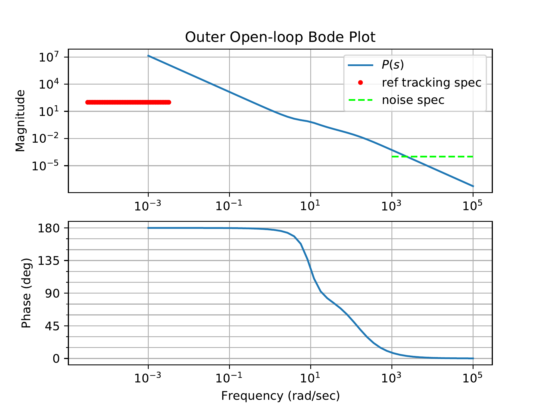
For the outer loop design, Fig.18.24
shows the Bode plot of the plant \(P=P_{out}\frac{P_{in}C_{in}}{1+P_{in}C_{in}}\)
together with the design specification on reference tracking and noise
attenuation.
Figure 18.24. The Bode plot for the outer loop plant in
HW 3.2.21, together with the
design specification.
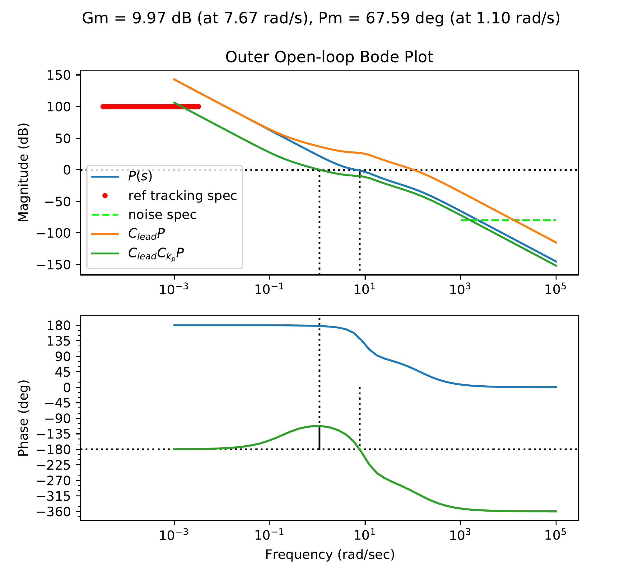
We want a rise time of 2 sec for the system, so this leads us to
select a crossover frequency of 1.1 rad/s. At 1.1 rad/s, the plant alone
has a small negative phase margin (remember that 180 deg and -180 deg
are equivalent), so to bring the phase margin up above 60 deg, we will
use a lead compensator centered at 1.1 rad/s with a lead ratio of 32 to
add 70 deg of phase. (A lead ratio of 32 is large. An alternative would
be to add two leads that each contribute 35 deg of phase margin.) As
shown in Fig.18.25,
with the lead applied, the crossover frequency is pushed out beyond
100 rad/s. By applying a proportional gain of 0.0146, we set the
crossover at 1.1 rad/s.
Figure 18.25. The Bode plot for the outer loop system
in HW 3.2.21, with lead compensation
and proportional gain.
As can be seen from Fig.18.25,
with the lead applied and crossover set at 1.1 rad/s, neither the
tracking constraint nor the noise attenuation constraint is satisfied.
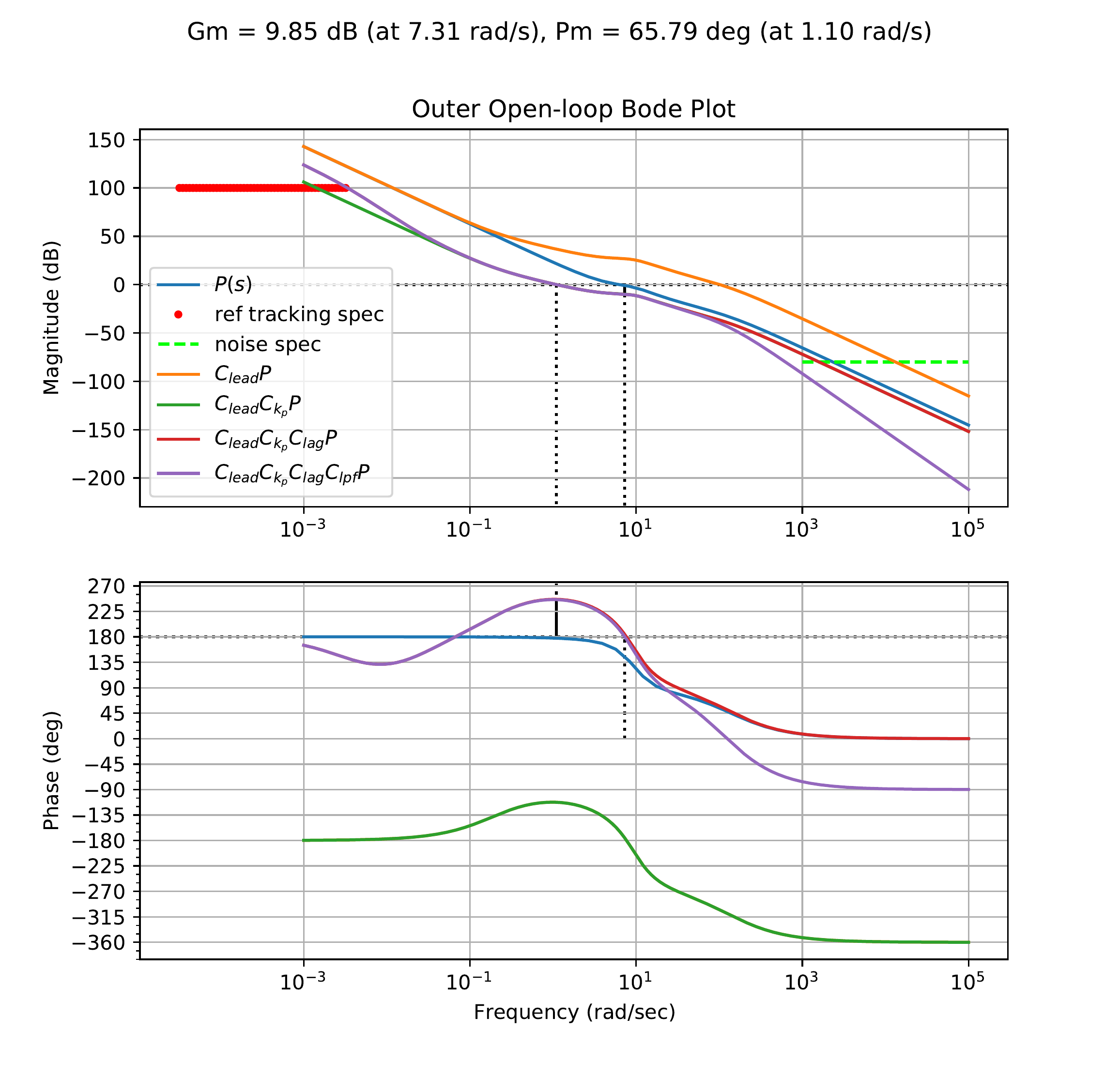
We can satisfy the tracking constraint by applying lag compensation to
boost the low-frequency gain near the constraint. Checking the gain of
the lead compensated system at the tracking constraint frequency (\(\omega_r\) = 0.0032 rad/s), we can see that
the gain is too low by a factor of 4.8. Applying a lag compensator with
a lag ratio of 8 ensures that this tracking constraint is satisfied as
shown in Fig.18.26.
Figure 18.26. The Bode plot for the outer loop system
in HW 3.2.21, with lead, and lag
control.
Finally, we can apply a low-pass filter to reduce the effects of
sensor noise in the system and satisfy the noise attenuation constraint.
To satisfy the constraint, we need to drop the gain of the open-loop
system by a factor of 2 at \(\omega_{no}\) = 1000 rad/s. We can
accomplish this with a low-pass filter with a cut-off frequency of
100 rad/s. This is shown in Fig.18.26
below. The resulting compensator is \[C_{out}(s) =
0.469\left(\frac{s+0.194}{s+6.24}\right)\left(\frac{s+0.0256}{s+0.0032}\right)\left(
\frac{100}{s+100} \right).\]
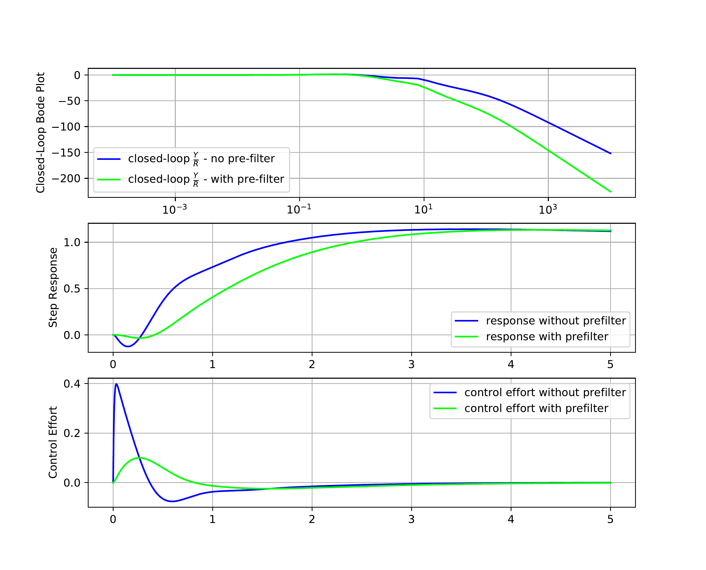
The closed-loop response for both the inner and outer loop systems,
as well as the unit-step responses for the output and control signal of
the outer loop, are all shown in Fig.18.27.
Figure 18.27. The closed-loop bode response, the
unit-step response for the output, and the unit step response for the
input of the inner loop design in HW 3.2.21.
A prefilter \[F(s) =
\frac{2}{s+2}\] has been added to the system. Note the
significant decrease in the control effort required when prefiltering is
used with the step input.
Python code that could be used to design the outer loop is shown
below. The Python code used to design the inner loop is shown below.
# 3rd-Partyimport numpy as npimport control as cntimport matplotlib.pyplot as plt# local (controlbook)import case_studies.B_pendulum.params as Pimport case_studies.common.loopshaping_tools as lsuse_dB =Falseplant_inner = cnt.tf(P.tf_inner_num, P.tf_inner_den)plant_outer = cnt.tf(P.tf_outer_num, P.tf_outer_den)############################################################# design controllers by loopshaping############################################################ ----------- inner loop -----------C_k_inner = ls.get_control_proportional(kp=-200.0)C_lead_inner = ls.get_control_lead(omega_lead=40.0, M=15.0)controller_inner = cnt.series(C_k_inner, C_lead_inner)sys_inner_ol = cnt.series(controller_inner, plant_inner)sys_inner_cl = cnt.feedback(sys_inner_ol, 1)# ----------- outer loop -----------# update the plant to include the inner loopplant_outer = cnt.series(sys_inner_cl, plant_outer)C_k_outer = ls.get_control_proportional(kp=0.023)C_lead_outer = ls.get_control_lead(omega_lead=1.0, M=18.0)C_lag_outer = ls.get_control_lag(z=0.04, M=5.0)C_lpf_outer = ls.get_control_lpf(p=50.0)controller_outer = cnt.series( C_k_outer, C_lead_outer, C_lag_outer, C_lpf_outer,)sys_outer_ol = cnt.series(controller_outer, plant_outer)sys_outer_cl = cnt.feedback(sys_outer_ol, 1)############################################################ add a prefilter to eliminate the overshoot###########################################################prefilter = ls.get_control_lpf(p=2.0)assert prefilter isnotNone# make type checkers happyif__name__=="__main__":############################################# inner loop############################################ w_lims = (1.0, 1e3) fig, ax = ls.plot_loopshape_stages( plant_inner, [ ("add proportional gain", C_k_inner), ("add lead", C_lead_inner), ],"Chapter 18 Loop Shaping: Pendulum on a Cart - Inner Loop", use_dB, omega_limits=w_lims, ) cnt.bode( sys_inner_cl, ax=ax, dB=use_dB, omega_limits=w_lims, grid=False, label="closed-loop", ) ax_mag = ax[0] ls.print_margins(sys_inner_ol, "Open-Loop (inner)", use_dB)# ----------- noise specification -------- omega_n =200.0 gamma_n =0.1 ls.draw_noise_spec(ax_mag, gamma_n, omega_n, use_dB)# ----------- bandwidth -------- bw_desired =40.0 bw_actual = cnt.bandwidth(sys_inner_cl) ax_mag.axvline(x=bw_actual, color="black", linestyle="-", label="bandwidth") ax_mag.axvline(x=bw_desired, color="red", linestyle="-.", label="bandwidth spec") ax_mag.legend(ncol=2, loc="lower left", fontsize="small") fig.tight_layout() plt.show()############################################# outer loop############################################ w_lims = (1e-3, 1e4) fig, ax = ls.plot_loopshape_stages( plant_outer, [ ("add proportional gain", C_k_outer), ("add lead", C_lead_outer), ("add lag", C_lag_outer), ("add low-pass filter", C_lpf_outer), ],"Chapter 18 Loop Shaping: Pendulum on a Cart - Outer Loop", use_dB, omega_limits=w_lims, )# cnt.bode(# sys_outer_cl,# ax=ax,# dB=use_dB,# omega_limits=w_lims,# grid=False,# label="closed-loop",# ) ax_mag = ax[0] ls.print_margins(sys_outer_ol, "Open-Loop (outer)", use_dB)# ----------- noise specification -------- omega_n =1000.0 gamma_n =0.0001 ls.draw_noise_spec(ax_mag, gamma_n, omega_n, use_dB)# ----------- tracking specification -------- omgega_r =0.0032 gamma_r =0.00001 ls.draw_ref_tracking_spec(ax_mag, gamma_r, omgega_r, use_dB)# ----------- crossover frequency -------- tr_des =2.0 wc_des =2.2/ tr_des# ax_mag.axvline(x=bw_actual, color="black", linestyle="-", label="bandwidth") ax_mag.axvline(x=wc_des, color="red", linestyle="-.", label=r"$\omega_c$ spec") ax_mag.legend(ncol=2, loc="lower left", fontsize="small") fig.tight_layout() plt.show()############################################# now check the closed-loop response with prefilter############################################# Closed loop transfer function from R to Y - no prefilter tf_R_to_Y_cl = cnt.feedback(sys_outer_ol, 1)# Closed loop transfer function from R to Y - with prefilter tf_R_to_Y_with_F_cl = cnt.series(prefilter, tf_R_to_Y_cl)# Closed loop transfer function from R to U - no prefilter tf_R_to_U_cl = cnt.feedback(controller_outer, plant_outer)# Closed loop transfer function from R to U - with prefilter tf_R_to_U_with_F_cl = cnt.series(prefilter, tf_R_to_U_cl) cnt.bode( [tf_R_to_Y_cl, tf_R_to_Y_with_F_cl], dB=use_dB,# plot_phase=False, label=[r"Closed-Loop $\frac{Y}{R}$ - no pre-filter",r"Closed-Loop $\frac{Y}{R}$ - with pre-filter", ], title="Closed-Loop Bode Plots: Pendulum on a Cart", ) plt.show()## Step response plots fig3, axes3 = plt.subplots(2, sharex=True) fig3.suptitle("Closed-Loop Step Responses: Pendulum on a Cart") tf =15.0 time = np.linspace(0, tf, 100) ax = axes3[0] _, y_out_no_F = cnt.step_response(tf_R_to_Y_cl, time) _, y_out_F = cnt.step_response(tf_R_to_Y_with_F_cl, time) ax.plot(time, y_out_no_F, label="no prefilter") ax.plot(time, y_out_F, label="with prefilter") ax.legend() ax.grid(True) ax.set_ylabel("Step Response") ax = axes3[1] _, u_out_no_F = cnt.step_response(tf_R_to_U_cl, time) _, u_out_F = cnt.step_response(tf_R_to_U_with_F_cl, time) ax.plot(time, u_out_no_F, label="no prefilter") ax.plot(time, u_out_F, label="with prefilter") ax.set_ylabel("Control Effort") ax.set_xlabel("Time (s)") ax.grid(True) plt.show()
For this homework assignment we will use the loopshaping design
technique to design a successive loop closure controller for the
satellite attitude problem.
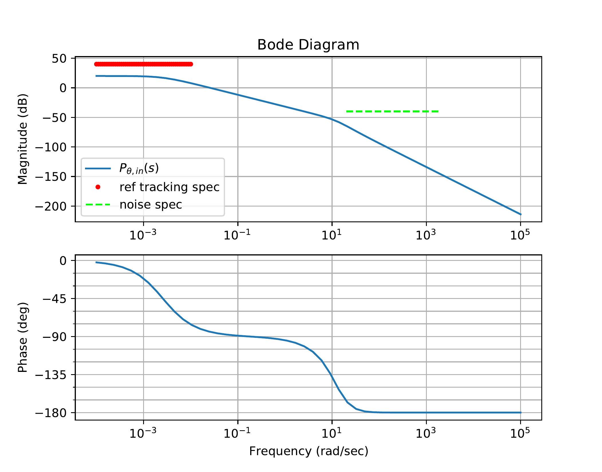
First consider the inner loop, where \(P_{in}(s)\) is the transfer function of the
inner loop derived in
HW 3.3.8. The Bode plot for
this system shows an underdamped resonant mode. We have seen in previous
chapters that this resonant mode can be removed by introducing rate
feedback of the form \[u = - k_D \dot{y} +
u',\] where \(y\) is the
output signal and \(u'\) is the
additional control signal to be designed. Using the derivative gain
\(k_{D_\theta}\) found in
HW 3.3.13, find the
revised transfer function from \(\tau'\) to \(\theta\), and use this transfer function
for \(P_{in}(s)\). Letting \[\tau'(s) = C_{in}(s) E(s),\] where
\(e(t) = \theta_r(t)-\theta(t)\),
design \(C_{in}(s)\) to meet the
following specifications:
The inner loop will track \(\theta_r\) with frequency content below
\(\omega_r=0.01\) radians/sec to within
\(\gamma_r=0.01\).
The inner loop will attenuate noise on the measurement of \(\theta\) for all frequencies above \(\omega_n=20\) rad/sec by \(\gamma_n=0.01\).
The phase margin of the inner loop should be around \(PM=60\) degrees.
Now consider the design of the controller for the outer-loop
system. As shown in HW 3.3.8, the transfer
function for the outer loop also has a strong resonant mode. As with the
inner loop, use the derivative gain found in
HW 3.3.13 to introduce
rate damping and find the associated transfer function \(P_{out}(s)\). The “plant” for the design of
the outer-loop controller is \[P =
P_{out}\frac{P_{in}C_{in}}{1+P_{in}C_{in}}.\] Design the outer
loop controller \(C_{out}\) to meet the
following specs:
Track steps in \(\phi_r\) with
zero steady-state error.
Reject input disturbances with frequency content below \(\omega_{d_{in}}=0.01\) by \(\gamma_{d_{in}}=0.1\).
Attenuate noise on the measurement of \(\phi\) with frequency content above \(\omega_n=10\) rad/sec by \(\gamma_n=10^{-4}\).
The phase margin of the outer loop should be around \(PM=60\) degrees.
Use a prefilter to reduce any peaking in the closed-loop response
of the outer loop.
Design Study C guided exercise
Plan satellite loop shaping
The satellite loop-shaping
design uses rate damping, inner-loop compensation, inner-loop collapse,
outer-loop compensation, and a prefilter.
Step 1. Inner-loop
plant preparation
Show solution for Step
1
Answer: Rate feedback damps the
inner plant; the worked inner compensator uses proportional gain and a
low-pass filter.
Step 2. Outer-loop
plant preparation
Show
solution for Step 2
Answer: The
outer-loop plant is \(P_{out}(P_{in}C_{in}/(1+P_{in}C_{in}))\), and
integral action is needed for zero steady-state error for a step
input.
Step 3. Final design
tradeoffs
Show solution for Step
3
Answer: The outer-loop design
uses lead/lag/filtering tradeoffs, and the prefilter reduces closed-loop
peaking in the reference response.
Pseudocode
Complete solution
From HW 3.3.8, the transfer
function model for the inner loop is given by \[\Theta(s) =
\frac{\frac{1}{J_s}}{s^2+\frac{b}{J_s}s+\frac{k}{J_s}}\tau(s).\]
Rate damping is added by designing the control signal so that \[\tau(s) = -k_D\frac{s}{\sigma s+1}\Theta(s) +
\tau'(s).\] Solving for \(\Theta(s)\) in terms of \(\tau'(s)\) gives \[\Theta(s) = \frac{\sigma s + 1}{\sigma J_s s^3 +
(\sigma b + J_s)s^2+(\sigma k + b + k_D)s + k}\tau'(s).\]
Therefore, for the inner loop we will set \[P_{in} = \frac{\sigma s + 1}{\sigma J_s s^3 +
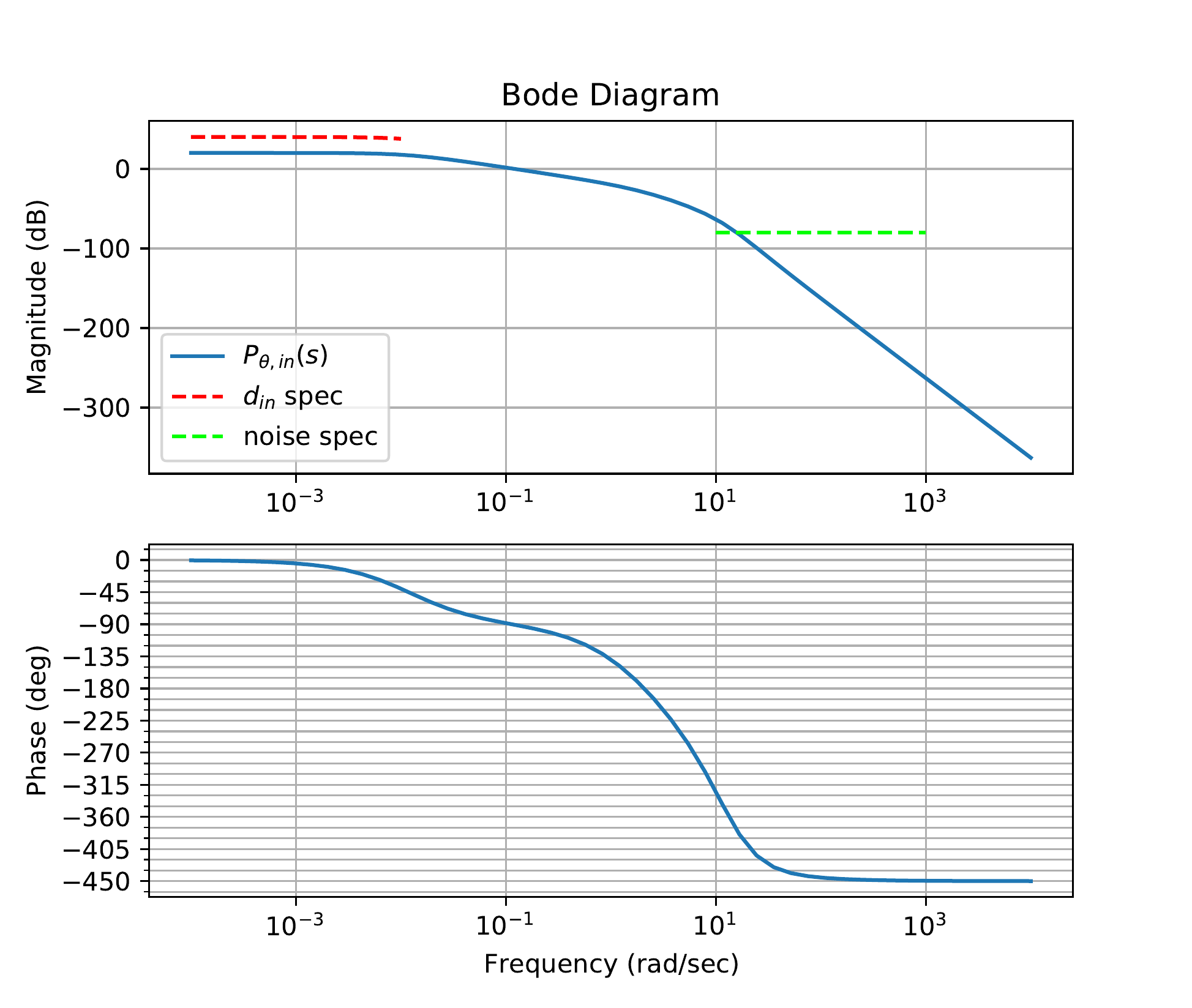
(\sigma b + J_s)s^2+(\sigma k + b + k_D)s + k}.\]Fig.18.28
shows the Bode plot of the plant \(P_{in}(s)\) together with the design
specification on input tracking and noise attenuation.
Figure 18.28. The Bode plot for the inner loop plant in
HW 3.3.21, together with the
design specification.
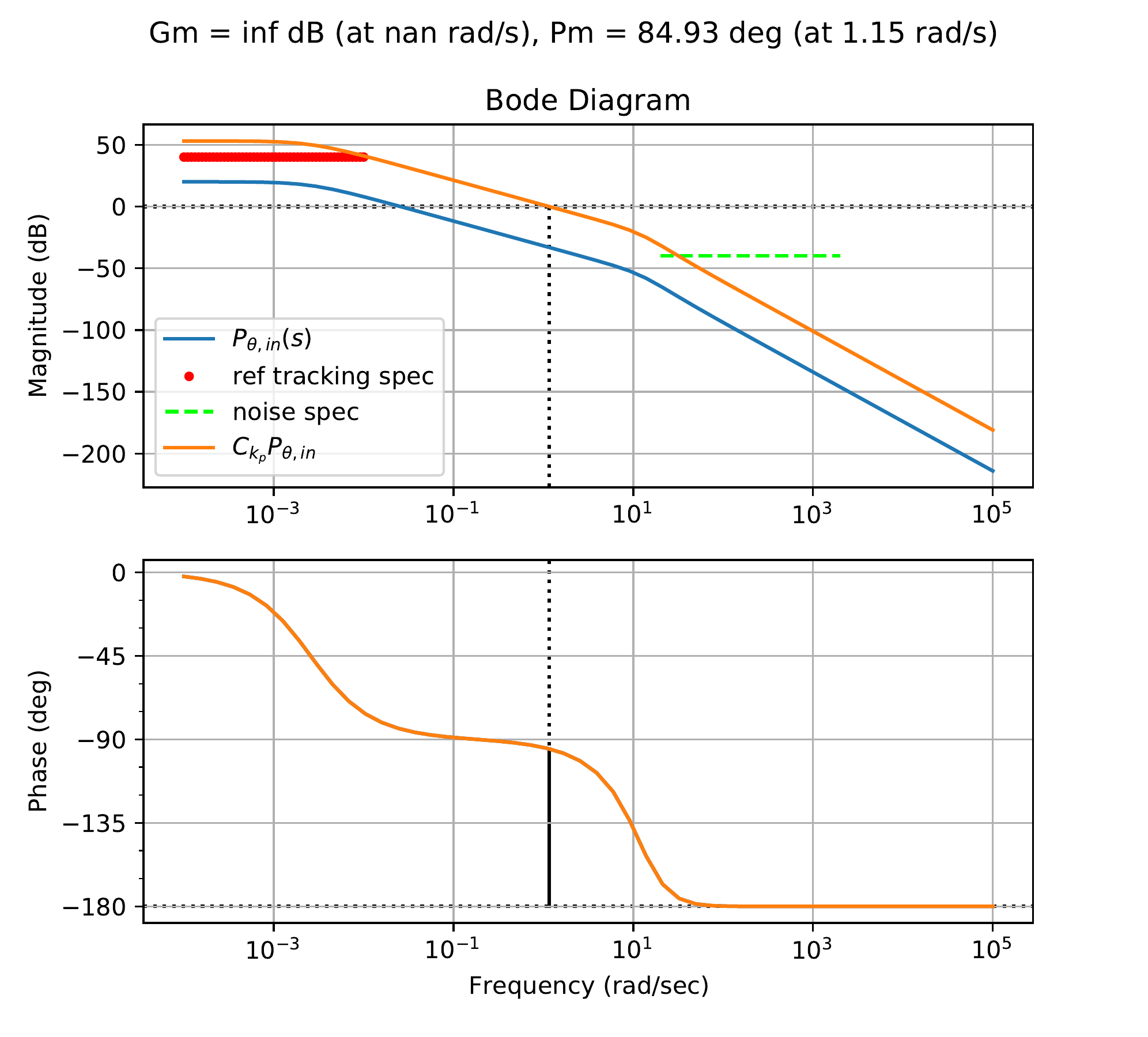
The first step is to add a proportional gain to satisfy the tracking
requirement. Fig.18.29
shows the corresponding Bode plot for a proportional gain of \(k_P=45\).
Figure 18.29. The Bode plot for the inner loop plant in
HW 3.3.21, with proportional
gain.
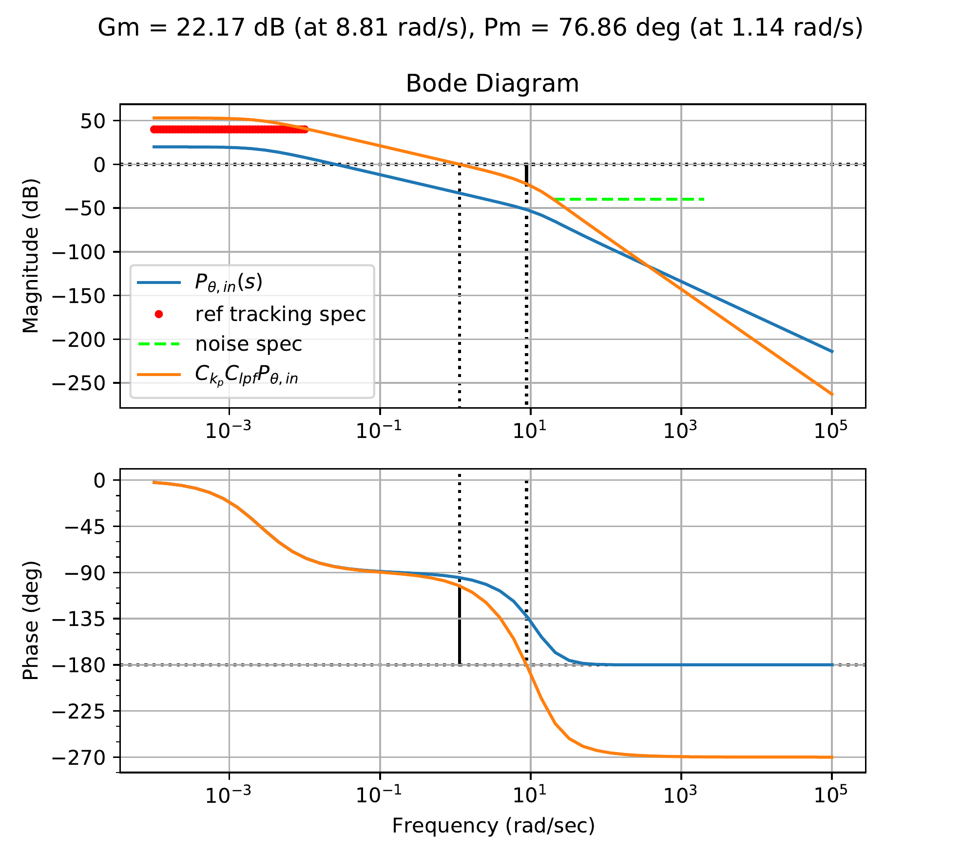
Since the phase margin is over \(PM=60\) degrees, a low-pass filter is
added. Fig.18.30
shows the loop gain with the addition of the low-pass filter \[C_{LPF} = \frac{8}{s+8},\] which has a
phase margin of \(PM=76.9\) degrees,
and satisfies the noise specification.
Figure 18.30. The Bode plot for the inner loop system
in HW 3.3.21, with proportional gain
and low-pass filter.
The resulting compensator is \[C_{in}(s) =
45\left(\frac{8}{s+8}\right).\] Notice that the DC gain is not
equal to one. The closed-loop response for the inner subsystem \[\frac{P_{in}C_{in}}{1+P_{in}C_{in}},\] as
well as the unit step response for the output and control signal are all
shown in Fig.18.31.
Figure 18.31. The closed-loop Bode response, the unit
step response for the output, and the unit step response for the input
of the inner loop design in HW 3.3.21.
The Python code used to design the inner loop is shown below.
The transfer function model for the outer loop was derived in HW 3.3.8 to be \[\Phi(s) =
\frac{\frac{b}{J_p}s+\frac{k}{J_p}}{s^2+\frac{b}{J_p}s+\frac{k}{J_p}}\Theta^r(s).\]
Rate damping is added by designing the control signal so that \[\Theta^r(s) = -k_D\frac{s}{\sigma s+1}\Phi(s) +
\Theta^{r'}(s).\] Solving for \(\Phi(s)\) in terms of \(\Theta^{r'}(s)\) gives \[\Phi(s) = \frac{\sigma b s^2 + (\sigma k + b)s +
k}{\sigma J_p s^3 + (\sigma b + J_p + bk_D)s^2+(\sigma k + b + kk_D)s +
k}\Theta^{r'}(s).\] The plant for the outer loop is therefore
\[P_{out} = \frac{\sigma s + 1}{\sigma J_p
s^3 + (\sigma b + J_p)s^2+(\sigma k + b + k_D)s +
k}\frac{P_{in}C_{in}}{1+P_{in}C_{in}}.\]Fig.18.32
shows the Bode plot for \(P_{out}\)
together with the design specification on rejecting input disturbances
and attenuating the noise. The requirement of zero steady-state error
for a step input requires a slope of \(-20\) dB/dec as \(s\to 0\) and is not shown in
Fig.18.32.
Figure 18.32. The Bode plot for the outer loop plant in
HW 3.3.21, together with the
design specifications.
The first step is to add an integrator to meet the steady-state
tracking requirement. The PM was also too low (\(PM=20.8\) degrees). So a lead compensator
is added at \(0.15\) rad/sec with \(M=120\), at approximately the midpoint in
frequency between the disturbance and noise constraints. This causes the
disturbance constraint to be violated. For this reason, a lag
compensator is also added to boost magnitude ratio at low frequencies.
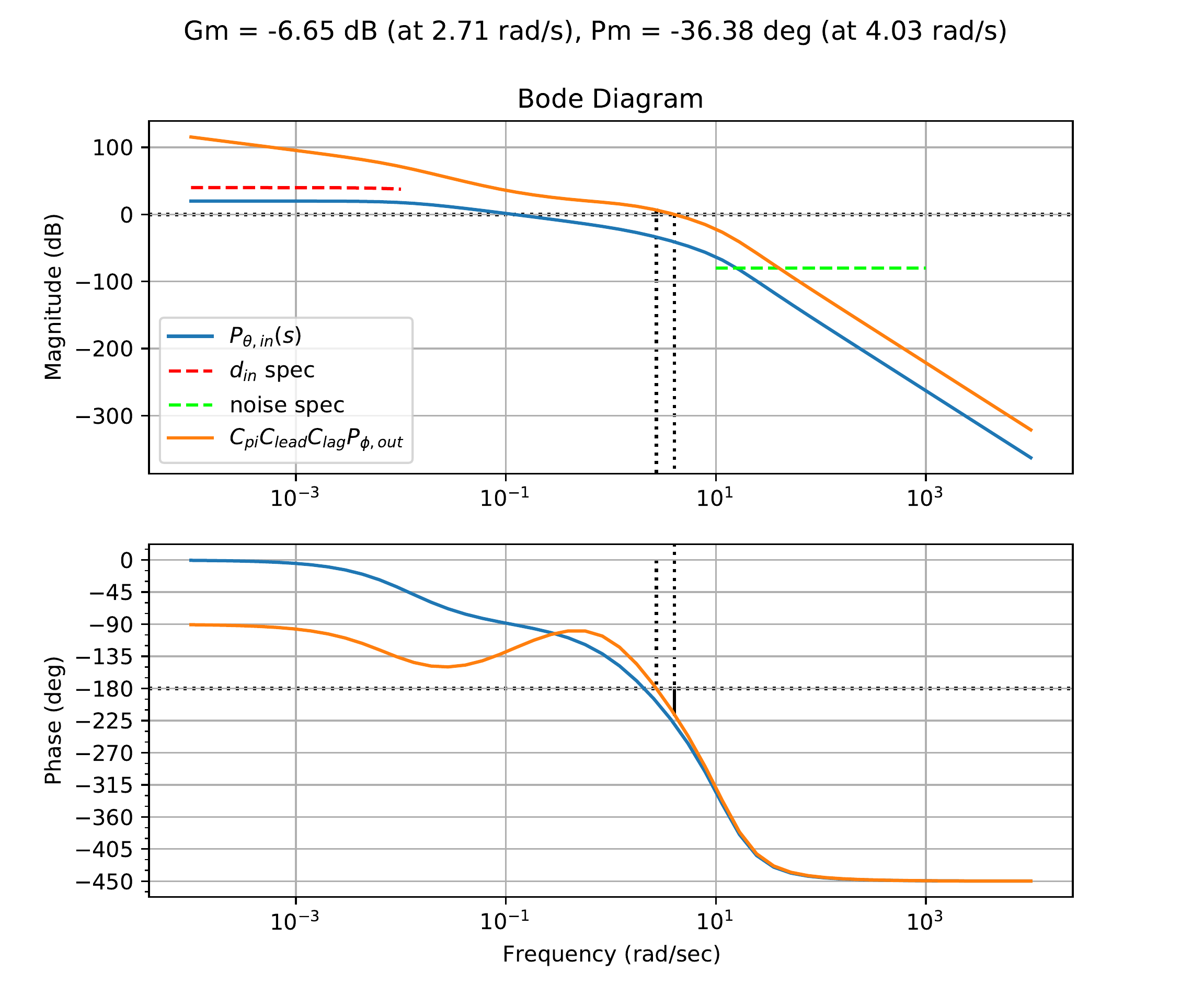
The lag compensator is defined with \(z=2.0\) and \(M=60.0\). Fig.18.33
shows the loop gain after adding the integral control, lead compensator,
and lag compensator. \[C =
C_{int}C_{lead}C_{lag}=\left(\frac{s+0.1}{s}\right)\left(\frac{120s +
1.64}{s + 1.64}\right)\left(\frac{s + 0.5}{0.0083}\right).\]
Figure 18.33. The Bode plot for the outer loop system
in HW 3.3.21, with integral, lead,
and lag control.
Without adding an overall gain to shift the crossover frequency
(i.e., to the desired \(0.15\) rad/sec
for which the lead compensator was designed), the phase margin shown in
Fig.18.33 is
\(PM=-36\) degrees. Therefore, a
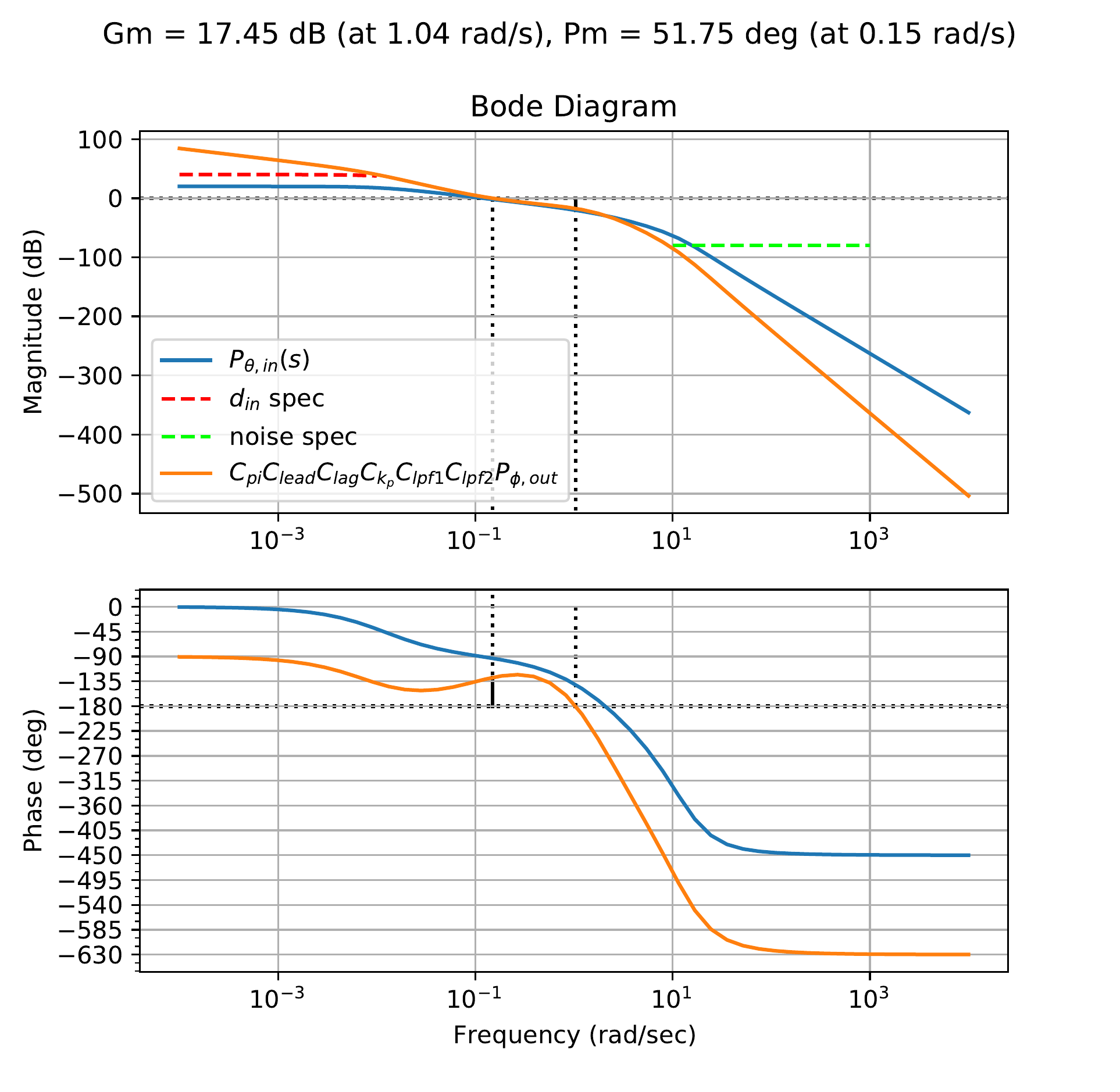
proportional gain of \(k_P=0.0275\) is
added to the compensator. Two low-pass filters with \(p=1.5\) and \(p=1.8\) are also added to meet the noise
constraint, and the result is shown in Fig.18.34.
The resulting system has \(PM=52\) degrees, which is a direct result
of tradeoffs between noise attenuation and tracking performance.
Figure 18.34. The Bode plot for the outer loop system
in HW 3.3.21, with the final
controller.
The final compensator is defined as: \[\begin{aligned}
C_{total} & = & C_{k_p} C_{pi}C_{lead} C_{lag}C_{lpf1}C_{lpf2}
\nonumber \\
& = & 0.0275\left(\frac{s+0.1}{s}\right)\left(\frac{120s +
1.64}{s + 1.64}\right)\left(\frac{s + 0.5}{0.0083}\right)\left(
\frac{1.5}{s + 1.5}\right)\left(\frac{1.8}{s+1.8}\right)\nonumber .
\end{aligned}\]
The closed-loop response for both the inner and outer loop systems,
as well as the unit step response for the output and control signal of
the outer loops, are all shown in Fig.18.35,
where the prefilter \[F(s) =
\frac{0.1}{s+0.1}\] has been added to reduce overshoot in the
closed-loop response.
Figure 18.35. The closed-loop Bode response, the unit
step response for the output, and the unit step response for the input
of the inner loop design in HW 3.3.21.
The time response of the outer loop is fairly slow, but this is
because of the chosen crossover frequency.
The Python code used to design the outer loop is shown below.
Tune real compensator blocks for
P(s)=1/(s+1). The Bode plot
shows how the controller changes the loop shape, and the checks below
connect the design to tracking, stability margin, bandwidth, and noise
attenuation requirements.
Interactive Figure 18.I5. The gray curve is
the plant, the blue curve is the compensated loop, the orange curve is
phase, and the green guides mark the design requirements.
Low-frequency
tracking
Phase margin
Bandwidth
Noise attenuation
Controller
Suggested next
move
18.6 Coding Lab: Compensator
Design
Objective: compose compensator
transfer-function blocks and score the resulting loop shape against
design requirements.
Evaluation
criteria: the lab checks low-frequency gain, high-frequency
rolloff, phase margin, properness, and stable compensator poles.
Figure 18.1 (Interactive). Compensator-design coding lab with
loop-shaping scorecard.
18.7 Knowledge Check
Q1.
Proportional gain effect
A
proportional gain primarily shifts the Bode magnitude:
Q2. Lead compensator purpose
A lead compensator is commonly used to add:
Q3. Gain combination
If two compensator blocks contribute +10 dB and -4 dB, enter the
combined magnitude contribution in dB.
Show solution
Answer: 6 dB. Bode magnitudes in dB add when
transfer-function blocks multiply.
Q4. Phase boost target
If the uncompensated phase margin is 30 degrees and the target is 60
degrees with a 20-degree safety allowance, enter the approximate phase
boost to design for.
Show solution
Answer: 50 degrees: 60 - 30 + 20 = 50 degrees.
Q5. Reference-response shaping
Which block can reduce reference-command overshoot without directly
changing loop stability margins?
Show solution
Answer: A prefilter shapes the reference path without
directly changing the loop gain PC.
Q6. Lead
block selection
Which compensator
block is the most direct choice when the design needs more positive
phase near crossover?
Q7. Lag block purpose
Why is a lag compensator commonly used in loop
shaping?
Q8. Low-pass filter purpose
What is the main loop-shaping role of a low-pass
filter?
Q9. Scorecard diagnosis
A design meets the low-frequency tracking
requirement but fails because phase margin is too small. What is the
most targeted next move?