P.4 Numerical Solutions to Differential Equations

This appendix provides a brief overview of techniques for numerically solving ordinary differential equations, when the initial value is specified. In particular, we are interested in solving the differential equation \[\tag{P.4.1} \dot{x} = \frac{dx}{dt}(t) = f(x(t), u(t)), \qquad x(t_0),\] over the time interval \([t_0, t_f]\), where \(x(t)\in \mathbf{R}^n\), and \(u(t)\in\mathbf{R}^m\) is assumed to be known, and where we assume that \(f(\cdot,\cdot)\) is sufficiently smooth and that unique solutions to the differential equation exist for every \(x_0\).

Integrating both sides of Equation P.4.1 from \(t_0\) to \(t<t_f\) gives \[\tag{P.4.2} x(t) = x(t_0) + \int_{t_0}^t f(x(\tau), u(\tau))\,d\tau.\] The difficulty with solving Equation P.4.2 is that \(x(t)\) appears on both sides of the equation, and cannot therefore be solved explicitly for \(x(t)\). All numerical solution techniques attempt to approximate the solution to Equation P.4.2. Most techniques break the solution into small time increments, usually equal to the sample rate of the computer, which we denote by \(T_s\). Accordingly we write Equation P.4.2 as \begin{align} x(t) &= x(t_0) + \int_{t_0}^{t-T_s} f(x(\tau), u(\tau))\,d\tau + \int_{t-T_s}^t f(x(\tau), u(\tau))\,d\tau \notag \\ &= x(t-T_s) + \int_{t-T_s}^t f(x(\tau), x(\tau))\,d\tau. \tag{P.4.3} \end{align}

The simplest form of numerical approximation for the integral in Equation P.4.3 is to use the left endpoint method, where \[\int_{t-T_s}^t f(x(\tau), u(\tau))\,d\tau \approx T_s f(x(t-T_s), u(t-T_s)).\] Using the notation \(x_k \stackrel{\triangle}{=}x(t_0+k T_s)\) we get the numerical approximation to the differential equation in Equation P.4.1 as \[\tag{P.4.4} x_k = x_{k-1} + T_s f(x_k, u_k), \quad x_0 = x(t_0).\] Equation P.4.4 is called the Euler method, or a Runge-Kutta first order method (RK1).

While the RK1 method is often effective for numerically solving ODEs, it typically requires a small sample size \(T_s\). The advantage of the RK1 method is that it only requires one evaluation of \(f(\cdot, \cdot)\).

To improve the numerical accuracy of the solution, a second-order method can be derived by approximating the integral in Equation P.4.3 using the trapezoidal rule shown in Figure 10.1, where \[\int_a^b f(\xi)d\xi \approx (b-a)\left(\frac{f(a)+f(b)}{2}\right).\] Accordingly, \[\int_{t-T_s}^t f(x(\tau), u(\tau))d\tau \approx \frac{T_s}{2}\left(f(x(t-T_s),u(t-T_s)) + f(x(t), u(t))\right).\] Since \(x(t)\) is unknown, we use the RK1 method to approximate it as \[x(t) \approx x(t-T_s) + T_s f(x(t-T_s), u(t-T_s)).\] In addition, we typically assume that \(u(t)\) is constant over the interval \([t-T_s, T_s)\) to get \[\begin{gathered} \int_{t-T_s}^t f(x(\tau), u(\tau))d\tau \approx \frac{T_s}{2}\big(f(x(t-T_s),u(t-T_s)) \\ + f(x(t-T_s) + T_s f(x(t-T_s), u(t-T_s)), u(t-T_s))\big). \end{gathered}\] Accordingly, the numerical integration routine can be written as \begin{align} x_0 &= x(t_0) \notag \\ F_1 &= f(x_{k-1}, u_{k-1}) \tag{P.4.5}\\ F_2 & = f(x_{k-1} + T_sF_1, u_{k-1}) \notag \\ x_k &= x_{k-1} + \frac{T_s}{2} \left( F_1 + F_2 \right). \notag \end{align} Equation P.4.5 is the Runge-Kutta second-order method, or RK2. It requires two function calls to \(f(\cdot, \cdot)\) for every time sample.

The most common numerical method for solving ODEs is the Runge-Kutta fourth order method RK4. The RK4 method is derived using Simpson’s Rule \[\int_a^b f(\xi)d\xi \approx \left(\frac{b-a}{6}\right)\left(f(a) + 4f\left(\frac{a+b}{2}\right) + f(b)\right),\] which is found by approximating the area under the integral using a parabola. The standard strategy is to write the approximation as \[\int_a^b f(\xi)\xi \approx \left(\frac{b-a}{6}\right)\left(f(a) + 2f\left(\frac{a+b}{2}\right) + 2f\left(\frac{a+b}{2}\right) + f(b)\right),\] and then to use \[\begin{aligned} F_1 &= f(a) \\ F_2 &= f( a + \frac{T_s}{2}F_1) \approx f\left(\frac{a+b}{2}\right)\\ F_3 &= f( a + \frac{T_s}{2}F_2) \approx f\left(\frac{a+b}{2}\right) \\ F_4 &= f( a + T_s F_3) \approx f(b), \end{aligned}\] resulting in the RK4 numerical integration rule \begin{align} x_0 &= x(t_0) \notag \\ F_1 &= f(x_{k-1}, u_{k-1}) \notag \\ F_2 & = f(x_{k-1} + \frac{T_s}{2} F_1, u_{k-1}) \tag{P.4.10} \\ F_3 & = f(x_{k-1} + \frac{T_s}{2} F_2, u_{k-1}) \notag \\ F_4 & = f(x_{k-1} + T_s F_3, u_{k-1}) \notag \\ x_k &= x_{k-1} + \frac{T_s}{6} \left( F_1 + 2F_2 + 2F_3 + F_4 \right). \notag \end{align}

It can be shown that the RK4 method matches the Taylor series approximation of the integral in Equation P.4.3 up to the fourth order term. Higher order methods can be derived, but generally do not result in significantly better numerical approximations to the ODE. The step size \(T_s\) must still be chosen to be sufficiently small to result in good solutions. It is also possible to develop adaptive step size solvers. For example, the ODE45 algorithm in MATLAB solves the ODE using both an RK4 and an RK5 algorithm. The two solutions are then compared and if they are sufficiently different, then the step size is reduced. If the two solutions are close, then the step size can be increased.

P.4.1 Python Implementation of Numerical ODE Solvers

In the following code example, we show how to implement a system that is described by the second-order differential equation \[\ddot{y} + a_1 \dot{y} + a_2 \sin y = b u,\] where \(a_1\), \(a_2\) and \(b\) are constant coefficients and \(u\) is the system input. The first step is to put the system into state-space form. Selecting the states as \[x =\begin{pmatrix} x_1 \\ x_2 \end{pmatrix} \stackrel{\triangle}{=}\begin{pmatrix} y \\ \dot{y} \end{pmatrix}\] and differentiating gives the state-space equations \[\begin{aligned} \begin{pmatrix} \dot{x}_1 \\ \dot{x}_2 \end{pmatrix} &= \begin{pmatrix} x_2 \\ -a_1 x_2 - a_2 \sin x_1 + b u \end{pmatrix} \\ y &= x_1, \end{aligned}\] which is in the form \[\begin{aligned} \dot{x} &= f(x,u) \\ y &= h(x, u). \end{aligned}\]

Python code that implements a class for this system is given below. The class has two external properties: the sample rate self.Ts and the state self.state. The constant coefficients are treated as internal properties known only to the system and are therefore labeled as self.a1, self.a2, and self.b. When the class is instantiated, the __init__ function is called; this function initializes the states with their initial conditions and initializes the system coefficients \(a_1\), \(a_2\), and \(b\). The external method update takes the system input \(u\) and returns the system output \(y\). The update function first propagates the system dynamics \(\dot{x} = f(x,u)\) using one of the Runge-Kutta methods. In the code below, the RK4 algorithm is used, but internal methods that implement the RK1, RK2, and RK4 methods are all shown for educational purposes. The RK methods each use the internal function self.f, which specifies the system dynamics \(\dot{x}=f(x,u)\). This function is system-dependent. The update function then computes the output \(y=h(x)\) by calling the internal function self.h, which is also system-dependent.

import numpy as np

class systemDynamics:
    #  Model the system yddot + a1*ydot + a2*sin(y) = b*u
    def __init__(self, Ts=0.01):
        self.Ts = Ts  # sample rate
        # Specify the initial condition
        y0 = 0.0  # y at time zero
        ydot0 = 0.0  # ydot at time zero
        self.state = np.array([
            [y0],
            [ydot0],
        ])  # state at time zero
        self.a1 = 2.0
        self.a2 = 2.0
        self.b = 4.0

    def update(self, u):
        # This is the external method that takes the input u and
        # returns the output y.
        self.rk4_step(u)  # propagate the state by one time sample
        y = self.h()  # return the corresponding output
        return y

    def rk1_step(self, u):
        # Integrate ODE using Runge-Kutta RK1 algorithm
        F1 = self.f(self.state, u)
        self.state += self.Ts * F1

    def rk2_step(self, u):
        # Integrate ODE using Runge-Kutta RK2 algorithm
        F1 = self.f(self.state, u)
        F2 = self.f(self.state + self.Ts / 2 * F1, u)
        self.state += self.Ts / 2 * (F1 + F2)

    def _rk4_step(self, u):
        # Integrate ODE using Runge-Kutta RK4 algorithm
        F1 = self.f(self.state, u)
        F2 = self.f(self.state + self.Ts / 2 * F1, u)
        F3 = self.f(self.state + self.Ts / 2 * F2, u)
        F4 = self.f(self.state + self.Ts * F3, u)
        self.state += self.Ts / 6 * (F1 + 2 * F2 + 2 * F3 + F4)

    def f(self, state, u):
        # Return xdot = f(x,u)
        x1 = state.item(0)
        x2 = state.item(1)
        xdot = np.array([
            [x2],
            [-self._a1 * x2 - self._a2 * np.sin(x1) + self._b * u],
            ])
        return xdot

    def h(self):
        # return the output equations y=h(x)
        x1 = self.state.item(0)
        y = np.array([
            [x1],
            ])
        return y

The system is simulated using the following Python code. The system is instantiated on line 13. The while loop in lines 20–28 updates the internal system at the sample rate T_s rather than at the plot rate T_plot. The input is specified as a square wave on line 23. The system is propagated one step forward using the input u on line 24.

import matplotlib.pyplot as plt
from signalGenerator import signalGenerator
from plotData import plotData
from systemDynamics import systemDynamics

# simulation parameters
Ts = 0.01  # sample rate of simulation
T_plot = 0.1  # plot update rate
t_start = 0.0  # start time of simulation
t_end = 20.0  # end time of simulation

# instantiate system and input classes
system = systemDynamics(Ts)
input = signalGenerator(amplitude=0.5, frequency=0.1)

# instantiate the simulation plots and animation
dataPlot = plotData()

t = t_start  # time starts at t0=0
while t < t_end:  # main simulation loop
    t_next_plot = t + T_plot
    while t < t_next_plot:
        u = input.square(t)
        y = system.update(u)
        t = t + Ts  # advance time by Ts
    # update animation and data plots
    dataPlot.update(t, system.state, u)
    plt.pause(0.0001)
    
# Keeps the program from closing until the user presses a button.
print('Press key to close')
plt.waitforbuttonpress()
plt.close()

P.4.2 MATLAB Implementation of Numerical ODE Solvers

MATLAB code that implements a class for the system defined in the previous section is given below. The class has five properties: the sample rate self.Ts, the state self.state, and the constant coefficients self.a1, self.a2, and self.b. When the class is instantiated, the constructor systemDynamics(Ts) is called, which is where the states are initialized with their initial conditions, and the system coefficients \(a_1\), \(a_2\), and \(b\) are initialized. The class method update takes as its input the system input \(u\) and returns the system output \(y\). The update function first propagates the system dynamics \(\dot{x} = f(x,u)\) using one of the Runge-Kutta methods. In the code below, the RK4 algorithm is used, but internal methods that implement the RK1, RK2, and RK4 methods are all shown for educational purposes. The RK methods each use the internal function self.f, which is where the system dynamics \(\dot{x}=f(x,u)\) are specified. This function is system-dependent. The update function then computes the output \(y=h(x)\) by calling the internal function self.h, which is also system-dependent.

classdef systemDynamics < handle
    properties
        Ts
        state
        a1
        a2
        b
    end
    methods
        %---constructor-------------------------
        function self = systemDynamics(Ts)
            self.Ts = Ts;  % sample rate
            y0 = 0;  % initial y
            ydot0 = 0;  % initial y_dot
            self.state = [y0; ydot0];  % initial state
            self.a1 = 2; % system parameters
            self.a2 = 2;
            self.b = 4;
        end
        %----------------------------
        function y = update(self, u)
            % external method that takes u as input
            % and returns y
            self.rk4_step(u);
            y = self.h();
        end
        function self = rk1_step(self, u)
            % Integrate ODE using Runge-Kutta RK1 algorithm
            F1 = self.f(self.state, u);
            self.state = self.state + self.Ts * F1;
        end
        function self = rk2_step(self, u)
            % Integrate ODE using Runge-Kutta RK2 algorithm
            F1 = self.f(self.state, u);
            F2 = self.f(self.state + self.Ts/2*F1, u);
            self.state = self.state + self.Ts/2 * (F1 + F2);
        end
        function self = rk4_step(self, u)
            % Integrate ODE using Runge-Kutta RK4 algorithm
            F1 = self.f(self.state, u);
            F2 = self.f(self.state + self.Ts/2*F1, u);
            F3 = self.f(self.state + self.Ts/2*F2, u);
            F4 = self.f(self.state + self.Ts*F3, u);
            self.state = self.state...
                + self.Ts/6 * (F1 + 2*F2 + 2*F3 + F4);
        end
        function xdot = f(self, state, u)
            % Return xdot = f(x,u), 
            x1 = state(1);
            x2 = state(2);
            xdot = [x2;...
                -self.a1*x2 - self.a2*sin(x2) + self.b*u];
        end
        function y = h(self)
            % return y = h(x)
            x1 = self.state(1);
            y = x1;
        end
    end
end

The system is simulated using the following MATLAB code. The system is instantiated on line 7. The while loop in lines 13–23 updates the internal system at the sample rate T_s rather than at the plot rate T_plot. The input is specified as a square wave on line 17. The system is propagated one step forward using the input u on line 18.

% simulation parameters
Ts = 0.01;  % sample rate
T_plot = 0.1;  % plot update rate
t_start = 0.0; % simulation start time
t_end = 10.0; % simulation end timm
% instantiate dynamics and plotter
system = systemDynamics(Ts);  
input = signalGenerator(0.5, 0.2);
dataPlot = dataPlotter();

% main simulation loop
t = t_start;  
while t < t_end  
    % Propagate dynamics in between plot samples
    t_next_plot = t + P.t_plot;
    while t < t_next_plot 
        u = input.square(t);  % input is a square wave
        y = system.update(u);  % Propagate the dynamics
        t = t + P.Ts; % advance time by Ts
    end
    % update data plots
    dataPlot.update(t, system.state, u);
end

P.4.3 Simulink Implementation of Numerical ODE Solvers

The Simulink engine implements a variety of different ODE solvers. The system dynamics are specified in an s-function. An s-function that implements the system described above is shown below.

function [sys,x0,str,ts,simStateCompliance]...
    = system_dynamics(t,x,u,flag)
switch flag
  % Initialization
  case 0
    [sys,x0,str,ts,simStateCompliance]...
        =mdlInitializeSizes();
  % Derivatives
  case 1
    sys=mdlDerivatives(t,x,u);
  % Update 
  case 2
    sys=mdlUpdate(t,x,u);
  % Outputs 
  case 3
    sys=mdlOutputs(t,x,u);
  % GetTimeOfNextVarHit 
  case 4
    sys=mdlGetTimeOfNextVarHit(t,x,u);
  % Terminate %
  case 9
    sys=mdlTerminate(t,x,u);
  % Unexpected flags %
  otherwise
    DAStudio.error(...
        'Simulink:blocks:unhandledFlag',...
        num2str(flag));

end

%
%==============================================
% mdlInitializeSizes
% Return the sizes, initial conditions, and 
%  sample times for the S-function.
%==============================================
%
function [sys,x0,str,ts,simStateCompliance]...
    =mdlInitializeSizes()

sizes = simsizes;

sizes.NumContStates  = 2;
sizes.NumDiscStates  = 0;
sizes.NumOutputs     = 1;
sizes.NumInputs      = 1;
sizes.DirFeedthrough = 0;
sizes.NumSampleTimes = 1;   

sys = simsizes(sizes);

% initialize the initial conditions%
y0 = 0;
ydot0 = 0;
x0  = [y0; ydot0];
% str is always an empty matrix
str = [];

% initialize the array of sample times
ts  = [0 0];
simStateCompliance = 'UnknownSimState';

%
%==============================================
% mdlDerivatives
% Return the derivatives for the continuous 
% states.
%==============================================
%
function sys=mdlDerivatives(t,x,u,P)
  x1 = x(1);
  x2 = x(2);
  xdot = [x2;...
          -self.a1*x2 - self.a2*sin(x2) + self.b*u];  
sys = xdot;
% end mdlDerivatives

%
%==============================================
% mdlUpdate
% Handle discrete state updates, sample time 
% hits, and major time step requirements.
%==============================================
%
function sys=mdlUpdate(t,x,u)

sys = [];

% end mdlUpdate

%
%==============================================
% mdlOutputs
% Return the block outputs.
%==============================================
%
function sys=mdlOutputs(t,x,u)
    x1 = x(1);
    y = x1;
sys = y;

% end mdlOutputs

%
%==============================================
% mdlGetTimeOfNextVarHit
%==============================================
%
function sys=mdlGetTimeOfNextVarHit(t,x,u)

sampleTime = 1;    
sys = t + sampleTime;

% end mdlGetTimeOfNextVarHit

%
%==============================================
% mdlTerminate
% Perform any end of simulation tasks.
%==============================================
%
function sys=mdlTerminate(t,x,u)

sys = [];

% end mdlTerminate

The state equations \(\dot{x}=f(x,u)\) are implemented in the function
mdlDerivatives on lines 70–75, and the output equation \(y=h(x)\) is implemented in the function mdlOutputs on lines 97–102. The system is initialized in mdlInitializeSizes on lines 38–61.

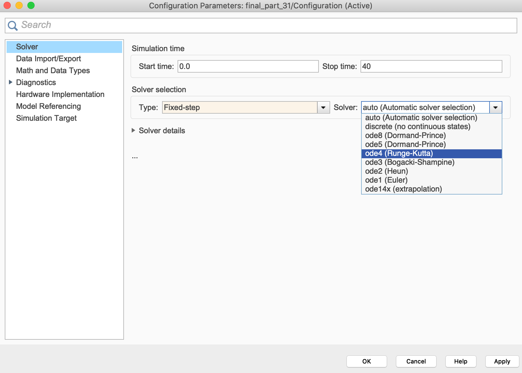
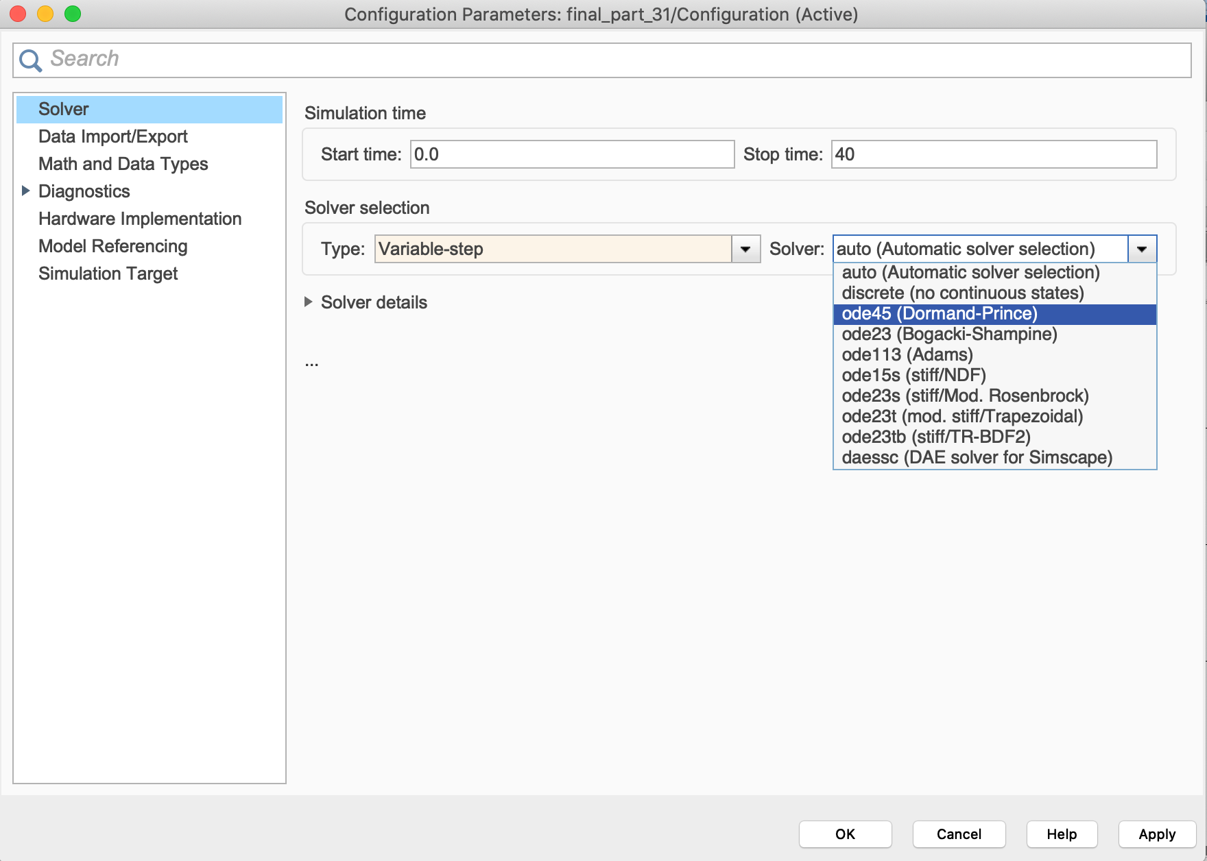
The numerical ODE solver can be specified by using the menu
Simulation > Model Configuration Parameters. Simulink has two types of solvers: fixed-step solvers and variable-step solvers. The dialog menu for fixed-step solvers is shown in Figure 4.1, where “ode4(Runge-Kutta)” corresponds to an RK4 method, “ode2(Heun)” corresponds to an RK2 method, and “ode1(Euler)” corresponds to an RK1 method. Simulink also has variable-step-size ODE solvers. The options for variable-step-size are shown in Figure 4.2. The “ode45 (Dormand-Prince)” solver works by solving the ODE over the next time step using both an ode4 and an ode5 method, comparing the two, and then reducing the step size if the difference is too large, and increasing the step size if the difference is within a tolerance.

P.4.4 Notes and References