In this chapter we show how the magnitude of the frequency response
of the open-loop system can be used to determine the performance of the
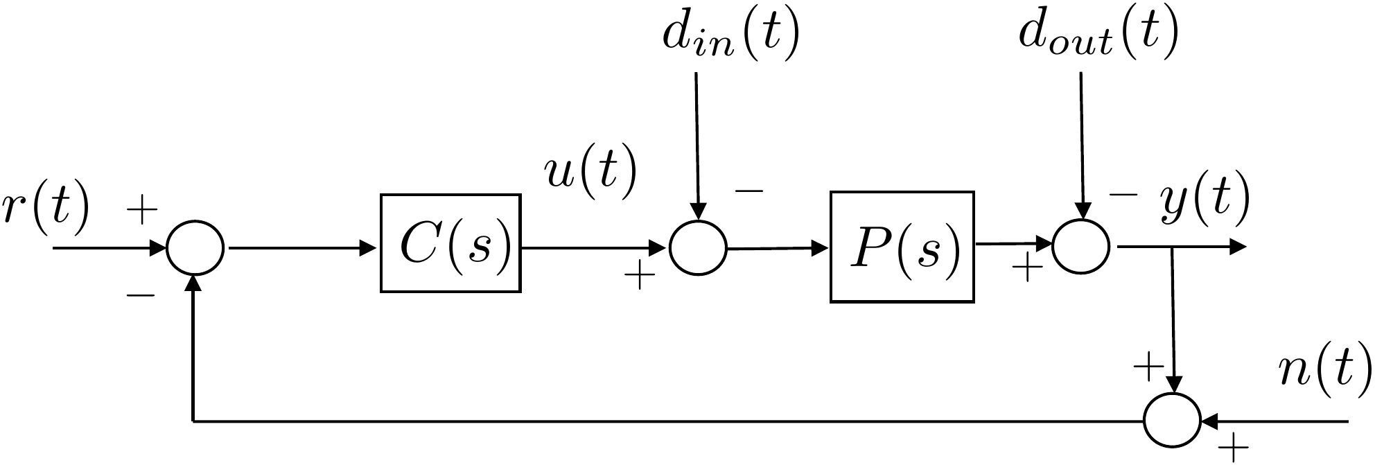
closed-loop feedback system. A general feedback
loop is shown in
Fig.16.1. In this feedback
system, \(r(t)\) is the reference input
to be tracked by \(y(t)\), \(d_{in}(t)\) is an unknown input
disturbance, \(d_{out}\) is an unknown output
disturbance, and \(n(t)\) is an unknown noise signal. Note that because of
the presence of \(n\), the error signal
\(e=r-y\) is no longer the input to
\(C(s)\). The input to \(C(s)\) is now \(r-y-n\). Note that this definition differs
from the one used in
Chapter 12 and will result in a
different transfer function between the error and the noise. To find the
transfer function from the inputs \(r\), \(d_{in}\), \(d_{out}\), and \(n\) to the error \(e(t)\) we start by finding the transfer
functions to \(y\). Starting at \(Y(s)\) and following the loop backward
until returning to \(Y\) we get \begin{align}
& Y(s) = -D_{out}(s) + P \left( - D_{in}(s) + C\left(R(s) - N(s) -
Y(s)\right) \right) \notag \\
\implies & (1+PC) Y(s) = PC R(s) - PC N(s) - D_{out}(s) - P
D_{in}(s) \notag \\
& Y(s) = \frac{PC}{1+PC}R(s) - \frac{PC}{1+PC} N(s)
%
- \frac{1}{1+PC} D_{out}(s) - \frac{P}{1+PC} D_{in}(s).
\tag{16.1}
\end{align} Defining the error to be \(E(s) \stackrel{\triangle}{=}R(s)-Y(s)\) we
get \begin{align}
E(s) &= R(s) - Y(s) \\
%
&= \frac{1}{1+PC}R(s) + \frac{PC}{1+PC} N(s)
%
+ \frac{1}{1+PC} D_{out}(s) + \frac{P}{1+PC} D_{in}(s),
\tag{16.3}
\end{align} Therefore,
The transfer function from the reference \(r\) to the error \(e\) is \(\frac{1}{1+P(s)C(s)}\),
The transfer function from the noise \(n\) to the error \(e\) is \(\frac{P(s)C(s)}{1+P(s)C(s)}\),
The transfer function from the output disturbance \(d_{out}\) to the error \(e\) is \(\frac{1}{1+P(s)C(s)}\), and
The transfer function from the input disturbance \(d_{in}\) to the error \(e\) is \(\frac{P(s)}{1+P(s)C(s)}\).
Figure 16.1. General feedback loop.
Chapter 16 activity
Trace the error transfer path
Select one input signal and follow how it appears in the error equation.
The highlighted path reinforces why different specifications use
different closed-loop transfer functions.
Figure 1.6.
The selected path shows which blocks determine the transfer function
from the chosen input to the error signal.
Selected
path
Transfer to error:
Specification
connection:
For typical applications, we have that
The reference signal \(r(t)\) is
a low frequency signal with frequency content below \(\omega_r\),
The noise signal \(n(t)\) is a
high frequency signal with frequency content above \(\omega_{\mathit{no}}\),
The output disturbance signal \(d_{out}(t)\) is a low frequency signal with
frequency content below \(\omega_{d_{out}}\),
The input disturbance signal \(d_{in}(t)\) is a low frequency signal with
frequency content below \(\omega_{d_{in}}\).
The objective for the control design is to find \(C(s)\) so that the following specifications
are satisfied:
Tracking: Track reference signals \(r(t)\) with frequency content below \(\omega_r\) so that the error due to the
reference signal satisfies \[\left|e(t)\right|\leq
\gamma_r\left|r(t)\right|,\]
Noise Attenuation: Attenuate noise signals \(n(t)\) with frequency content above \(\omega_{no}\) so that the error due to the
noise signal satisfies \[\left|e(t)\right|\leq
\gamma_n\left|n(t)\right|,\]
Reject Output Disturbances: Reject output
disturbance signals \(d_{out}(t)\) with
frequency content below \(\omega_{d_{out}}\) so that the error due to
the output disturbance signal satisfies \[\left|e(t)\right|\leq
\gamma_{d_{out}}\left|d_{out}(t)\right|,\]
Reject Input Disturbances: Reject input
disturbance signals \(d_{in}(t)\) with
frequency content below \(\omega_{d_{in}}\) so that the error due to
the input disturbance signal satisfies \[\left|e(t)\right|\leq
\gamma_{d_{in}}\left|d_{in}(t)\right|.\]
The objective in the remainder of this chapter is to show how each of
these specifications can be translated into a requirement on the
magnitude of the (open) loop gain \(20\log_{10}\left|P(j\omega)C(j\omega)\right|\).
16.1.1 Tracking
The transfer function
from the reference signal \(r(t)\) to
the error \(e(t)\) is \[E(s) = \frac{1}{1+P(s)C(s)}R(s).\]
Therefore, \[\left|E(j\omega)\right| \leq
\left|\frac{1}{1+P(j\omega)C(j\omega)}\right|\left|R(j\omega)\right|.\]
The objective is to track reference signals \(r(t)\) with frequency content below \(\omega_r\) so that the error due to the
reference signal satisfies \[\left|e(t)\right|\leq \gamma_r
\left|r(t)\right|.\] Therefore, the controller \(C(s)\) needs to be designed so that \[\left|\frac{1}{1+P(j\omega)C(j\omega)}\right|
\leq \gamma_r,\] or equivalently so that \[\left|1+P(j\omega)C(j\omega)\right| \geq
\frac{1}{\gamma_r}.\] If \(\left|P(j\omega)C(j\omega)\right|\gg 1\),
then a sufficient condition is that \[\left|P(j\omega)C(j\omega)\right| \geq
\frac{1}{\gamma_r},\] or equivalently \[\tag{16.4}
20\log_{10}\left|P(j\omega)C(j\omega)\right| \geq
20\log_{10}1/\gamma_r,\] which needs to be satisfied for all
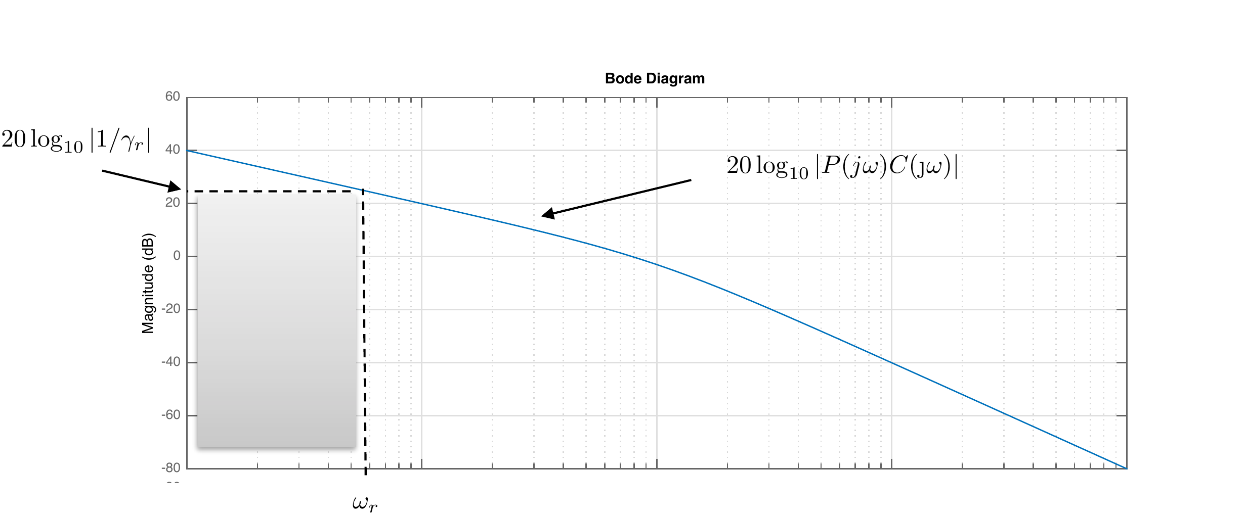
\(\omega\leq\omega_r\). On a Bode plot,
the constraint represented by
Equation 16.4
is shown graphically in
Fig.16.2.
Figure 16.2. Bode plot representation of the
loop-shaping constraint corresponding to tracking r(t) so that the
corresponding error satisfies |e(t)| ≤ γr|r(t)|.
Alternatively, from the Bode plot of \(PC\) we can compute the tracking
characteristics of the closed-loop system. For example, suppose that on
the Bode plot \[20\log_{10}\left|P(j\omega)C(j\omega)\right|>
B_r\text{~dB}\] for all \(\omega<\omega_r\), then \[\left|P(j\omega)C(j\omega)\right|>
10^{B_r/20},\] for all \(\omega<\omega_r\). If \(\left|P(j\omega)C(j\omega)\right|\gg 1\)
for all \(\omega<\omega_r\), then
\[\left|\frac{1}{1+P(j\omega)C(j\omega)}\right|\lessapprox
10^{-B_r/20},\] which implies that \[\left|E(j\omega)\right| \leq 10^{-B_r/20}
\left|R(j\omega)\right|\] for all \(\omega<\omega_r\), or in other words
that \[\tag{16.5}
\left|e(t)\right| \leq 10^{-B_r/20} \left|r(t)\right|,\] for all
\(r(t)\) with frequency content below
\(\omega_r\), which implies that \[\gamma_r = 10^{-B_r/20}.\]
16.1.2 Noise Attenuation
The transfer function from the noise signal \(n(t)\) to the error \(e(t)\) is \[E(s)
= \frac{P(s)C(s)}{1+P(s)C(s)}N(s).\] Therefore, \[\left|E(j\omega)\right| \leq
\left|\frac{P(j\omega)C(j\omega)}{1+P(j\omega)C(j\omega)}\right|\left|N(j\omega)\right|.\]
The objective is to attenuate noise signals \(n(t)\) with frequency content above \(\omega_{no}\) so that the error due to the
noise signal satisfies \[\left|e(t)\right|\leq \gamma_n
\left|n(t)\right|.\] Therefore, the controller \(C(s)\) needs to be designed so that \[\left|\frac{P(j\omega)C(j\omega)}{1+P(j\omega)C(j\omega)}\right|
\leq \gamma_n.\] If \(\left|P(j\omega)C(j\omega)\right|\ll 1\),
then a sufficient condition is that \[\left|P(j\omega)C(j\omega)\right| \leq
\gamma_n,\] or equivalently \[\tag{16.6}
20\log_{10}\left|P(j\omega)C(j\omega)\right| \leq
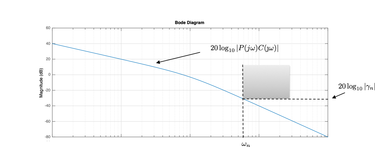
20\log_{10}\gamma_n,\] which needs to be satisfied for all \(\omega\geq\omega_{no}\). On a Bode plot,
the constraint represented by
Equation 16.6
is shown graphically in
Fig.16.3.
Figure 16.3. Bode plot representation of the
loop-shaping constraint corresponding to attenuating the noise n(t) so that the
corresponding error satisfies |e(t)| ≤ γn|n(t)|.
Alternatively, from the Bode plot of \(PC\) we can compute the noise attenuation
characteristics of the closed-loop system. For example, suppose that on
the Bode plot \[20\log_{10}\left|P(j\omega)C(j\omega)\right|<
-B_n\text{~dB}\] for all \(\omega>\omega_{no}\), then \[\left|P(j\omega)C(j\omega)\right|<
10^{-B_n/20},\] for all \(\omega>\omega_{no}\). If \(P(j\omega)C(j\omega)\ll 1\) for all \(\omega>\omega_{no}\), then \[\left|\frac{P(j\omega)C(j\omega)}{1+P(j\omega)C(j\omega)}\right|\lessapprox
10^{-B_n/20},\] which implies that \[\left|E(j\omega)\right| \leq 10^{-B_n/20}
\left|N(j\omega)\right|\] for all \(\omega>\omega_{no}\), or in other words
that \[\left|e(t)\right| \leq 10^{-B_n/20}
\left|n(t)\right|,\] for all \(n(t)\) with frequency content above \(\omega_{no}\), which implies that \[\gamma_n = 10^{-B_n/20}.\]
16.1.3 Reject Output
Disturbances
The transfer function
from the output disturbance signals \(d_{out}(t)\) to the error \(e(t)\) is \[E(s)
= \frac{1}{1+P(s)C(s)}D_{out}(s).\] Therefore, \[\left|E(j\omega)\right| \leq
\left|\frac{1}{1+P(j\omega)C(j\omega)}\right|\left|D_{out}(j\omega)\right|.\]
The objective is to attenuate output disturbance signals \(d_{out}(t)\) with frequency content below
\(\omega_{d_{out}}\) so that the error
due to the output disturbance signal satisfies \[\left|e(t)\right|\leq \gamma_{d_{out}}
\left|d_{out}(t)\right|.\] Therefore, the controller \(C(s)\) needs to be designed so that \[\left|\frac{1}{1+P(j\omega)C(j\omega)}\right|
\leq \gamma_{d_{out}},\] or equivalently so that \[\left|1+P(j\omega)C(j\omega)\right| \geq
\frac{1}{\gamma_{d_{out}}}.\] If \(\left|P(j\omega)C(j\omega)\right|\gg 1\),
then a sufficient condition is that \[\left|P(j\omega)C(j\omega)\right| \geq
\frac{1}{\gamma_{d_{out}}},\] or equivalently \[\tag{16.7}
20\log_{10}\left|P(j\omega)C(j\omega)\right| \geq
20\log_{10}1/\gamma_{d_{out}},\] which needs to be satisfied for
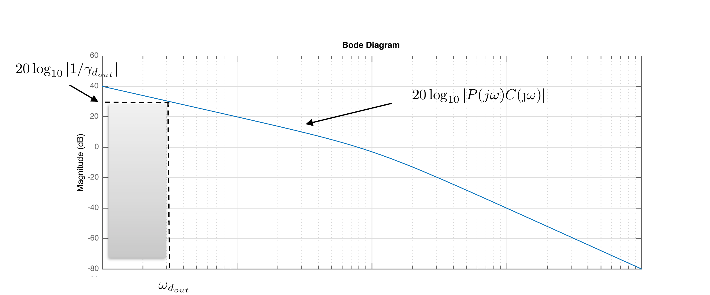
all \(\omega\leq\omega_{d_{out}}\). On
a Bode plot, the constraint represented by
Equation 16.7
is shown graphically in
Fig.16.4.
Figure 16.4. Bode plot representation of the
loop-shaping constraint corresponding to rejecting the output
disturbance dout(t)
so that the corresponding error satisfies |e(t)| ≤ γdout|dout(t)|.
Alternatively, from the Bode plot of \(PC\) we can compute the output disturbance
rejection characteristics of the closed-loop system. For example,
suppose that on the Bode plot \[20\log_{10}\left|P(j\omega)C(j\omega)\right|>
B_{d_{out}}\text{~dB}\] for all \(\omega<\omega_{d_{out}}\), then \[\left|P(j\omega)C(j\omega)\right|>
10^{B_{d_{out}}/20},\] for all \(\omega<\omega_{d_{out}}\). If \(\left|P(j\omega)C(j\omega)\right|\gg 1\)
for all \(\omega<\omega_{d_{out}}\),
then \[\left|\frac{1}{1+P(j\omega)C(j\omega)}\right|\lessapprox
10^{-B_{d_{out}}/20},\] which implies that \[\left|E(j\omega)\right| \leq 10^{-B_{d_{out}}/20}
\left|D_{out}(j\omega)\right|\] for all \(\omega<\omega_{d_{out}}\), or in other
words that \[\left|e(t)\right| \leq
10^{-B_{d_{out}}/20} \left|d_{out}(t)\right|,\] for all \(d_{out}(t)\) with frequency content below
\(\omega_{d_{out}}\), which implies
that \[\gamma_{d_{out}} =
10^{-B_{d_{out}}/20}.\]
16.1.4 Reject Input
Disturbances
The transfer function
from the input disturbance signals \(d_{in}(t)\) to the error \(e(t)\) is \[E(s)
= \frac{P(s)}{1+P(s)C(s)}D_{in}(s).\] Therefore, \[\left|E(j\omega)\right| \leq
\left|\frac{P(j\omega)}{1+P(j\omega)C(j\omega)}\right|\left|D_{in}(j\omega)\right|.\]
The objective is to attenuate input disturbance signals \(d_{in}(t)\) with frequency content below
\(\omega_{d_{in}}\) so that the error
due to the input disturbance signal satisfies \[\left|e(t)\right|\leq \gamma_{d_{in}}
\left|d_{in}(t)\right|.\] Therefore, the controller \(C(s)\) needs to be designed so that \[\left|\frac{P(j\omega)}{1+P(j\omega)C(j\omega)}\right|
\leq \gamma_{d_{in}},\] or equivalently so that \[\frac{\left|1+P(j\omega)C(j\omega)\right|}{\left|P(j\omega)\right|}
\geq \frac{1}{\gamma_{d_{in}}}.\] If \(\left|P(j\omega)C(j\omega)\right|\gg 1\),
then a sufficient condition is that \[\frac{\left|P(j\omega)C(j\omega)\right|}{\left|P(j\omega)\right|}
\geq \frac{1}{\gamma_{d_{in}}},\] or equivalently \[\tag{16.8}
20\log_{10}\left|P(j\omega)C(j\omega)\right| -
20\log_{10}\left|P(j\omega)\right| \geq
20\log_{10}1/\gamma_{d_{in}},\] which needs to be satisfied for
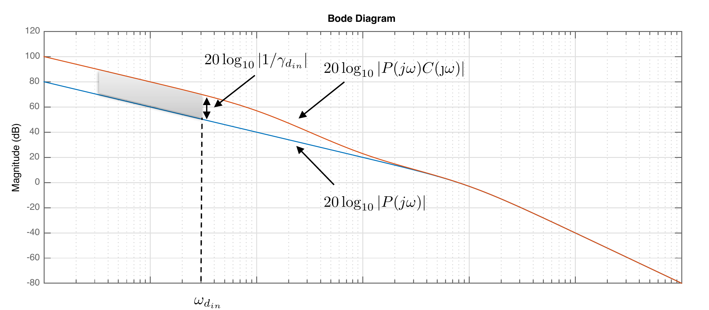
all \(\omega\leq\omega_{d_{in}}\). On a
Bode plot, the constraint represented by
Equation 16.8
is shown graphically in
Fig.16.5, where it can be
seen that the loop gain \(\left|PC\right|\) must be above the
magnitude of the plant \(\left|P\right|\) by the specified
amount.
Figure 16.5. Bode plot representation of the
loop-shaping constraint corresponding to rejecting the input disturbance
din(t)
so that the corresponding error satisfies |e(t)| ≤ γdin|din(t)|.
Alternatively, from the Bode plot of \(PC\) we can compute the input disturbance
rejection characteristics of the closed-loop system. For example,
suppose that on the Bode plot \[20\log_{10}\left|P(j\omega)C(j\omega)\right|-20\log_{10}\left|P(j\omega)\right|>
B_{d_{in}}\text{~dB}\] for all \(\omega<\omega_{d_{in}}\), then \[\frac{\left|P(j\omega)C(j\omega)\right|}{\left|P(j\omega)\right|}>
10^{B_{d_{in}}/20},\] for all \(\omega<\omega_{d_{in}}\). If \(\left|P(j\omega)C(j\omega)\right|\gg 1\)
for all \(\omega<\omega_{d_{in}}\),
then \[\left|\frac{P(j\omega)}{1+P(j\omega)C(j\omega)}\right|\lessapprox
10^{-B_{d_{in}}/20},\] which implies that \[\left|E(j\omega)\right| \leq 10^{-B_{d_{in}}/20}
\left|D_{in}(j\omega)\right|\] for all \(\omega<\omega_{d_{in}}\), or in other
words that \[\tag{16.9}
\left|e(t)\right| \leq 10^{-B_{d_{in}}/20}
\left|d_{in}(t)\right|,\] for all \(d_{in}(t)\) with frequency content below
\(\omega_{d_{in}}\), which implies that
\[\gamma_{d_{in}} =
10^{-B_{d_{in}}/20}.\]
16.1.5 Frequency Response
Characterization of System Type
Recall that the loop gain \(P(s)C(s)\) is said to be
Type 0 if there are no free integrators,
Type 1 if there is one free integrator,
Type 2 if there are two free integrators, etc.
15.1.5.1 Type 0 System
Note that for a type 0 system \[\begin{aligned}
& \lim_{s\to 0} P(s)C(s) = \text{~constant} \\
\implies & \lim_{\omega\to 0}\left|P(j\omega)C(j\omega)\right| =
\text{~constant} \\
\implies & \lim_{\omega\to 0}
20\log_{10}\left|P(j\omega)C(j\omega)\right| = \text{~constant}.
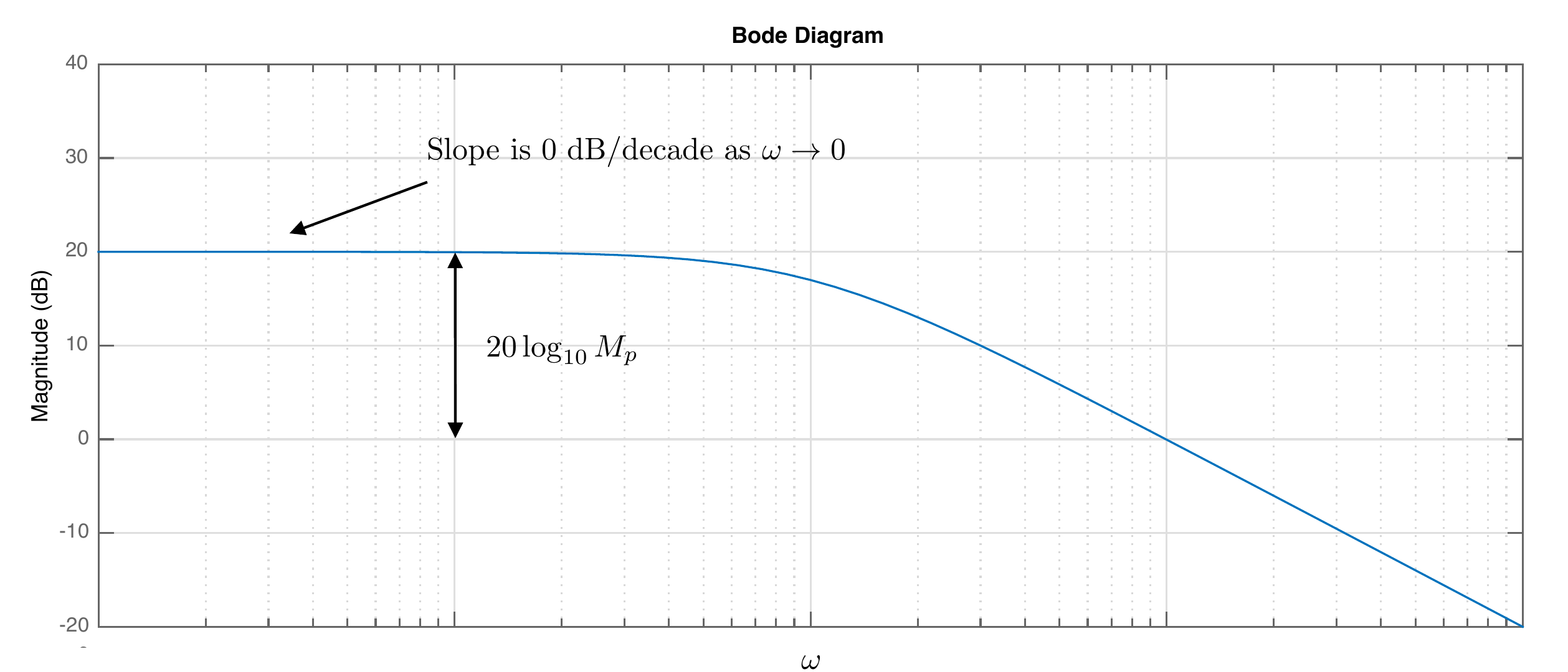
\end{aligned}\] In other words, at low frequency, the Bode
magnitude plot is as shown in
Fig.16.6.
Figure 16.6. Bode plot of a type 0
system.
Recall that for a step input to a type 0 system where \(R(s) = A/s\), the steady-state error is
\[e_{ss} = \lim_{t\to \infty} e(t) =
\lim_{s\to 0} sE(s) = \lim_{s\to 0} \frac{A}{1+P(s)C(s)} =
\frac{A}{1+M_p},\] where \[M_p =
\lim_{s\to 0}P(s)C(s) = \lim_{\omega\to 0}
\left|P(j\omega)C(j\omega)\right|.\] As shown in
Fig.16.6, \(20\log_{10}M_p\) is the constant limit of
the loop gain as \(\omega\to 0\).
Therefore, from the Bode plot of \(PC\) for a type 0 system, we can compute
the tracking error for a step input of size \(A\). Suppose that on the Bode plot \[\lim_{\omega\to 0}
20\log_{10}\left|P(j\omega)C(j\omega)\right| = B_0\text{~dB}.\]
Then \[M_p = 10^{B_0/20},\] and \[\tag{16.10}
\lim_{t\to\infty}\left|e(t)\right| \leq \frac{1}{1+M_p} A.\]
15.1.5.2 Type 1 System
For a type 1 system since \(P(s)C(s)\) has one free integrator \[\begin{aligned}
& \lim_{s\to 0} sP(s)C(s) = \text{~constant} \\
\implies & \lim_{\omega\to
0}\left|(j\omega)P(j\omega)C(j\omega)\right| = \text{~constant} \\
\implies & \lim_{\omega\to
0}\frac{\left|P(j\omega)C(j\omega)\right|}{\left|\frac{1}{j\omega}\right|}
= \text{~constant} \\
\implies & \lim_{\omega\to 0} \left[
20\log_{10}\left|P(j\omega)C(j\omega)\right| -
20\log_{10}\left|\frac{1}{j\omega}\right|\right] = \text{~constant}.
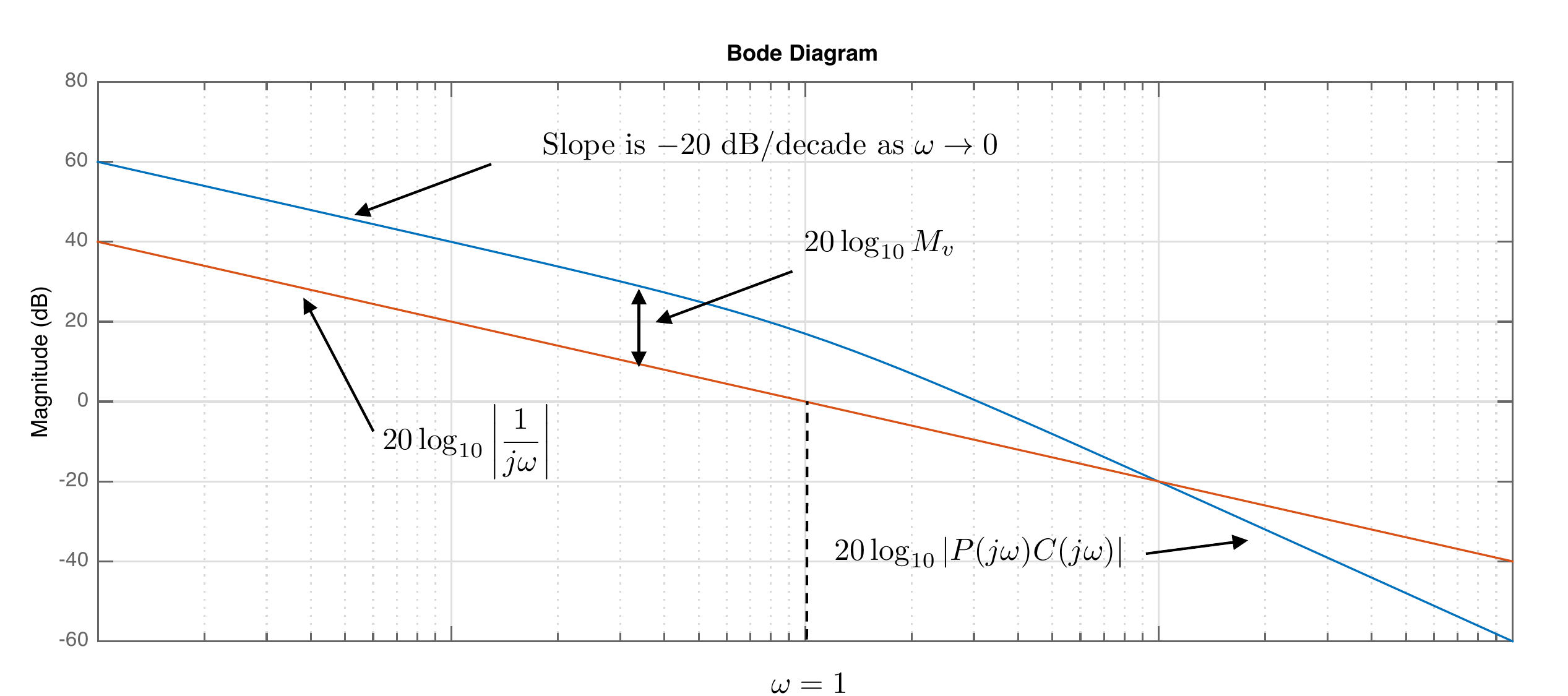
\end{aligned}\] In other words, at low frequency, the Bode
magnitude plot of \(20\log_{10}\left|P(j\omega)C(j\omega)\right|\)
has a slope of \(-20\) dB/decade as
\(\omega\to 0\), as shown in
Fig.16.7.
Figure 16.7. Bode plot of a type 1
system.
Recall that for a ramp input to a type 1 system where \(R(s) = A/s^2\), the steady-state error is
\[e_{ss} = \lim_{t\to \infty} e(t) =
\lim_{s\to 0} sE(s) = \lim_{s\to 0} \frac{A}{s+sP(s)C(s)} =
\frac{A}{M_v},\] where \[M_v =
\lim_{s\to 0}sP(s)C(s) = \lim_{\omega\to 0}
\left|(j\omega)P(j\omega)C(j\omega)\right|.\] As shown in
Fig.16.7, \(20\log_{10}M_v\) is the amount that the
loop gain exceeds the Bode plot of \(20\log_{10}\left|1/j\omega\right|\) as
\(\omega\to 0\).
Therefore, from the Bode plot of \(PC\) for a type 1 system, we can compute
the tracking error for a ramp input with slope \(A\). Suppose that on the Bode plot \[\lim_{\omega\to 0} \left[
20\log_{10}\left|P(j\omega)C(j\omega)\right| -
20\log_{10}\left|\frac{1}{j\omega}\right| \right] =
B_1\text{~dB},\] then \[M_v =
10^{B_1/20},\] and \[\tag{16.11}
\lim_{t\to\infty}\left|e(t)\right| \leq \frac{1}{M_v} A.\]
15.1.5.3 Type 2 System
For a type 2 system where \(P(s)C(s)\) has two free integrators we have
\[\begin{aligned}
& \lim_{s\to 0} s^2P(s)C(s) = \text{~constant} \\
\implies & \lim_{\omega\to
0}\left|(j\omega)^2P(j\omega)C(j\omega)\right| = \text{~constant} \\
\implies & \lim_{\omega\to
0}\frac{\left|P(j\omega)C(j\omega)\right|}{\left|\frac{1}{j\omega}\right|^2}
= \text{~constant} \\
\implies & \lim_{\omega\to 0} \left[
20\log_{10}\left|P(j\omega)C(j\omega)\right| -
20\log_{10}\left|\frac{1}{j\omega}\right|^2\right] = \text{~constant}.
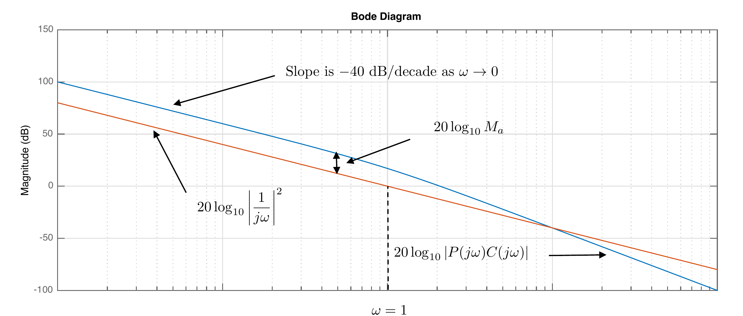
\end{aligned}\] In other words, at low frequency, the Bode
magnitude plot of \(20\log_{10}\left|P(j\omega)C(j\omega)\right|\)
has a slope of \(-40\) dB/decade as
\(\omega\to 0\), as shown in
Fig.16.8.
Figure 16.8. Bode plot of a type 2
system.
Recall that for a parabolic input to a type 2 system where \(R(s) = A/s^3\), the steady-state error is
\[e_{ss} = \lim_{t\to \infty} e(t) =
\lim_{s\to 0} sE(s) = \lim_{s\to 0} \frac{A}{s^2+s^2P(s)C(s)} =
\frac{A}{M_a},\] where \[M_a =
\lim_{s\to 0}s^2P(s)C(s) = \lim_{\omega\to 0}
\left|(j\omega)^2P(j\omega)C(j\omega)\right|.\] As shown in
Fig.16.8, \(20\log_{10}M_a\) is the amount that the
loop gain exceeds the Bode plot of \(20\log_{10}\left|1/j\omega\right|^2\) as
\(\omega\to 0\).
Therefore, from the Bode plot of \(PC\) for a type 2 system, we can compute
the tracking error for a parabola input with curvature \(A\). Suppose that on the Bode plot \[\lim_{\omega\to 0} \left[
20\log_{10}\left|P(j\omega)C(j\omega)\right| -
20\log_{10}\left|\frac{1}{j\omega}\right|^2 \right] =
B_2\text{~dB}.\] Then \[M_a =
10^{B_2/20},\] and \[\tag{16.12}
\lim_{t\to\infty}\left|e(t)\right| \leq \frac{1}{M_a} A.\]
Chapter 16 activity
Measure system type from the low-frequency slope
Use two markers to measure the low-frequency slope of
|L(jω)|. The slope tells you
how many free integrators are in the loop: 0, 1, or 2. After classifying
the type, choose an input class to estimate the corresponding
steady-state error constant.
Step 1: measure the low-frequency slope
Place both
markers on the low-frequency straight-line part of the Bode magnitude
curve.
Slope-to-type reference:0 dB/decade →
Type 0-20 dB/decade → Type 1-40
dB/decade → Type 2
Figure 1.7. Use the two
markers to estimate the low-frequency slope. After the type is
classified correctly, the orange guide shows the input class used to
measure the relevant error constant.
Step 2: estimate the steady-state error
The input size
A scales the final error. It
does not move the Bode curve. After the type is classified, compare
|L(jω)|
with the selected input-class guide to estimate Mp, Mv, or Ma.
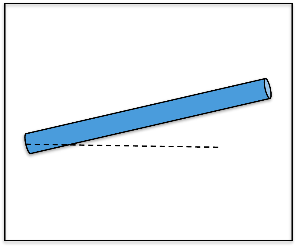
For the single-link robot arm, use the bode command
(from MATLAB or Python) to create a graph that simultaneously displays
the Bode plots for (1) the plant, (2) the plant under PID control, using
the control gains calculated in
HW 3.1.13.
(a) To what percent error can the closed-loop system under PID control track
the desired input if all of the frequency content of \(\theta_r(t)\) is below \(\omega_r = 0.4\) radians per second?
(b) If the reference input is \(\theta_r(t) =
5t^2\) for \(t\geq 0\), what
will the steady-state tracking error to this input be when using PID
control?
(c) If all of the frequency content of the input disturbance \(d_{in}(t)\) is below \(\omega_{d_{in}} = 0.01\) radians per
second, what percentage of the input disturbance shows up in the output
\(\theta\) under PID control?
(d) If all of the frequency content of the noise \(n(t)\) is greater than \(\omega_{no} = 100\) radians per second,
what percentage of the noise shows up in the output signal \(\theta\)?
Design Study A guided exercise
Measure frequency-domain specifications
Read tracking,
disturbance, and noise bounds as frequency-specific magnitude
requirements.
Use the
marked Bode plot to read the frequency and magnitude values used in the
specification checks.
Step 1. Tracking specification variables
Show solution for
Step 1
Answer: The acceptable
tracking region is specified by a frequency \(\omega_r\) and a magnitude bound \(\gamma_r\).
Step 2. Convert magnitude bound to percent
Show solution for
Step 2
Answer: A magnitude error
bound \(\gamma_r\) corresponds to
approximately \(100\gamma_r%\).
Step 3. Identify high and low-frequency specs
Show solution for Step
3
Answer: Disturbance rejection is
a low-frequency requirement, while sensor-noise attenuation is a
high-frequency requirement.
Complete solution
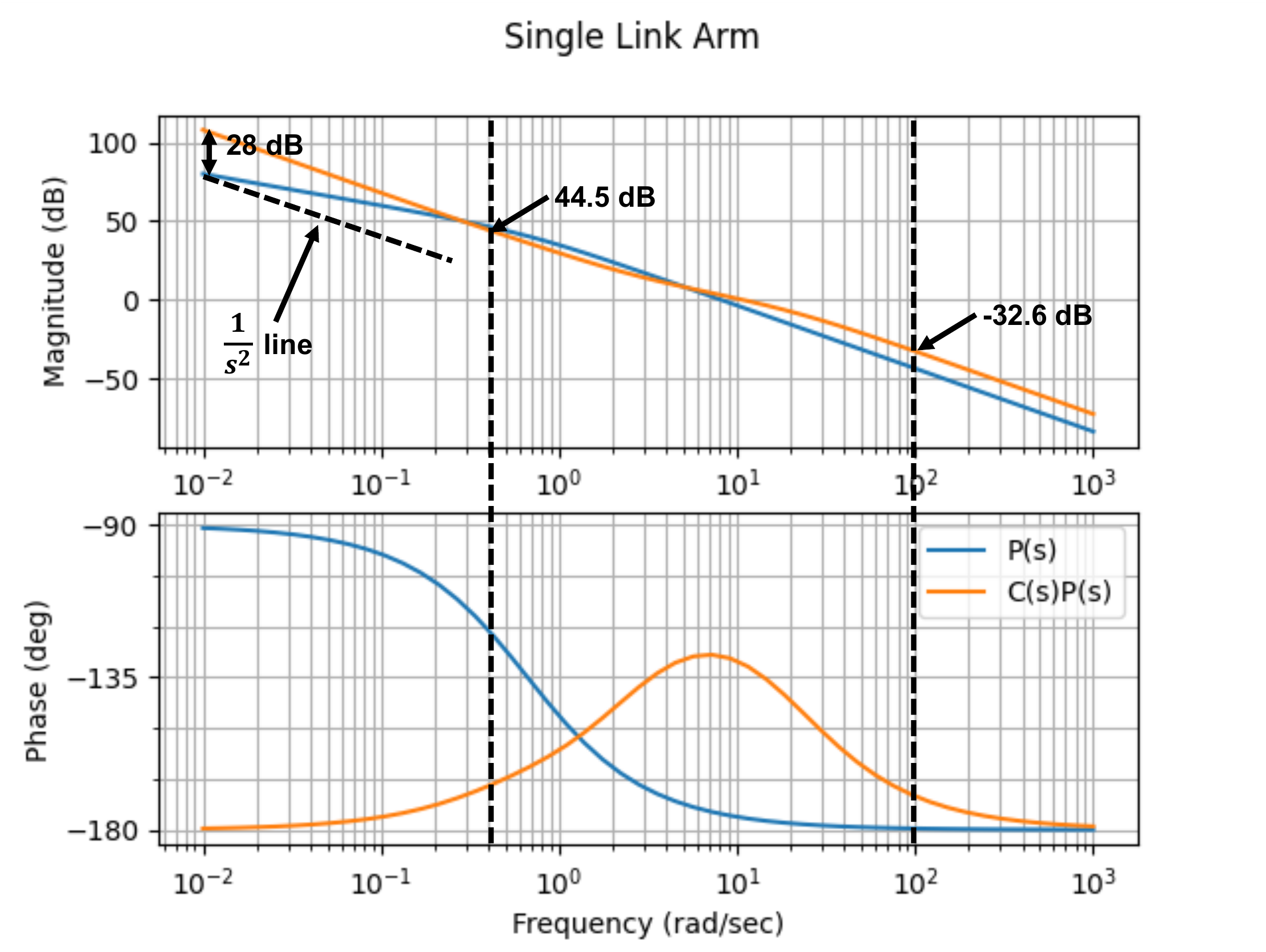
(a) The Bode plots of the plant \(P(s)\) and the loop gain with PID control
\(P(s)C_{PID}(s)\) are shown in
Fig.16.9.
Figure 16.9. Bode plot for single-link robot arm,
plant only and under PID control.
From Fig.16.9 we see that below \(\omega_r = 0.4\) rad/sec, the loop gain is
above \(B_r=44.5\) dB. Therefore, from
Equation 16.5 we have
that \[\left|e(t)\right| \leq \gamma_r
\left|r(t)\right|,\] where \(\gamma_r =
10^{-44.5/20} = 0.006\), which implies that the tracking error
will be 0.60% of the magnitude of the input.
(b) Suppose now that the desired reference input is
\(\theta_r(t) = 5t^2\). Under PID
control, the slope of the loop gain as \(\omega\to 0\) is \(-40\) dB/dec, which implies that the system
is type 2 and will track a step and a ramp with zero steady-state error.
For a parabola, there will be a finite error. Since the loop gain under
PID control is \(B_2=28\) dB above the
\(1/s^2\) line, from Equation 16.12
the steady-state error satisfies \[\lim_{t\to\infty}\left|e(t)\right| \leq
\frac{A}{M_a} = 5\cdot 10^{-28/20} = 0.2.\]
(c) If the input disturbance is below \(\omega_{d_{in}} = 0.01\) rad/s, then the
difference between the loop gain and the plant is \(B_{d_{in}}=28\) dB at \(\omega_{d_{in}} = 0.01\) rad/s, therefore,
from Equation 16.9
we see that \[\gamma_{d_{in}} = 10^{-28/20} =
0.04,\] implying that 4% of the input disturbance will show up in
the output.
(d) For noise greater than \(\omega_{no}=100\) rad/sec, we see from
Fig.16.9 that \(B_n = 32.6\) dB. Therefore, \(\gamma_n = 10^{-32.6/20} = 0.023\) which
implies that \(2.3\)% of the noise will
show up in the output signal.
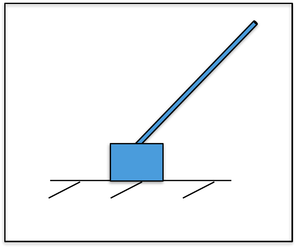
For the inner loop of the inverted pendulum, use the
bode command (in Python or MATLAB) to create a graph that
simultaneously displays the Bode plots for (1) the plant, and (2) the
plant under PD control, using the control gains calculated in
Homework 3.2.13.
(a) To what percent error can the closed-loop system track the desired input
if all of the frequency content of \(\theta_r(t)\) is below \(\omega_r = 1.0\) radians per second?
(b) If all of the frequency content of the sensor noise on the inner \(n(t)\) is greater than \(\omega_{no} = 200\) radians per second,
what percentage of the noise shows up in the output signal \(\theta\)?
For the outer loop of the inverted pendulum, use the MATLAB
bode command to create a graph that simultaneously displays
the Bode plots for the plant, and the plant under PID control, using the
control gains calculated in
Homework 3.2.13.
(c) If the reference signal \(y_r(t)\) has
frequency content below \(\omega_r=0.001\) radians/second, what is
the tracking error under PID control if \(\left|r(t)\right|\leq 50\)?
Design
Study B guided exercise
Read pendulum frequency-domain
specs
Use Bode-plot bounds to estimate tracking and noise
attenuation.
Use the markers to connect dB bounds to
tracking and noise percentages.
Step 1. Inner-loop tracking frequency
Show solution for Step
1
Answer: The inner-loop tracking
specification is evaluated below omega_r = 1 rad/s.
Step 2.
Inner-loop noise frequency
Show
solution for Step 2
Answer: The
inner-loop noise specification is evaluated above omega_no = 200
rad/s.
Step 3.
Outer-loop reference frequency
Show
solution for Step 3
Answer: The
outer-loop tracking bound is evaluated below omega_r = 0.001
rad/s.
Complete solution
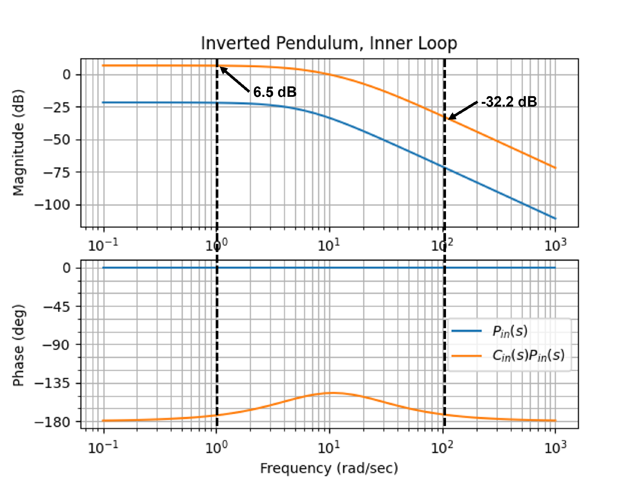
(a) The Bode plots of the plant \(P(s)\) and the loop gain with PD control
\(P(s)C_{PD}(s)\) are shown in
Fig.16.10.
Figure 16.10. Bode plot for the inner loop of the
inverted pendulum for (1) plant only (blue), and (2) under PD control
(orange).
From Fig.16.10 we see that
below \(\omega_r = 1.0\) rad/sec, the
loop gain is above \(B_r=6.5\) dB.
Therefore, from Equation 16.5 we have
that \[\left|e(t)\right| \leq \gamma_r
\left|r(t)\right|,\] where \(\gamma_r =
10^{-6.5/20} = 0.47\), which implies that the tracking error will
be 47% of the magnitude of the input.
(b) For noise greater than \(\omega_{no}=200\) rad/sec, we see from
Fig.16.10 that \(B_n = 32.2\) dB. Therefore, \(\gamma_n = 10^{-32.2/20} = 0.0245\) which
implies that \(2.45\)% of the noise
will show up in the output signal.
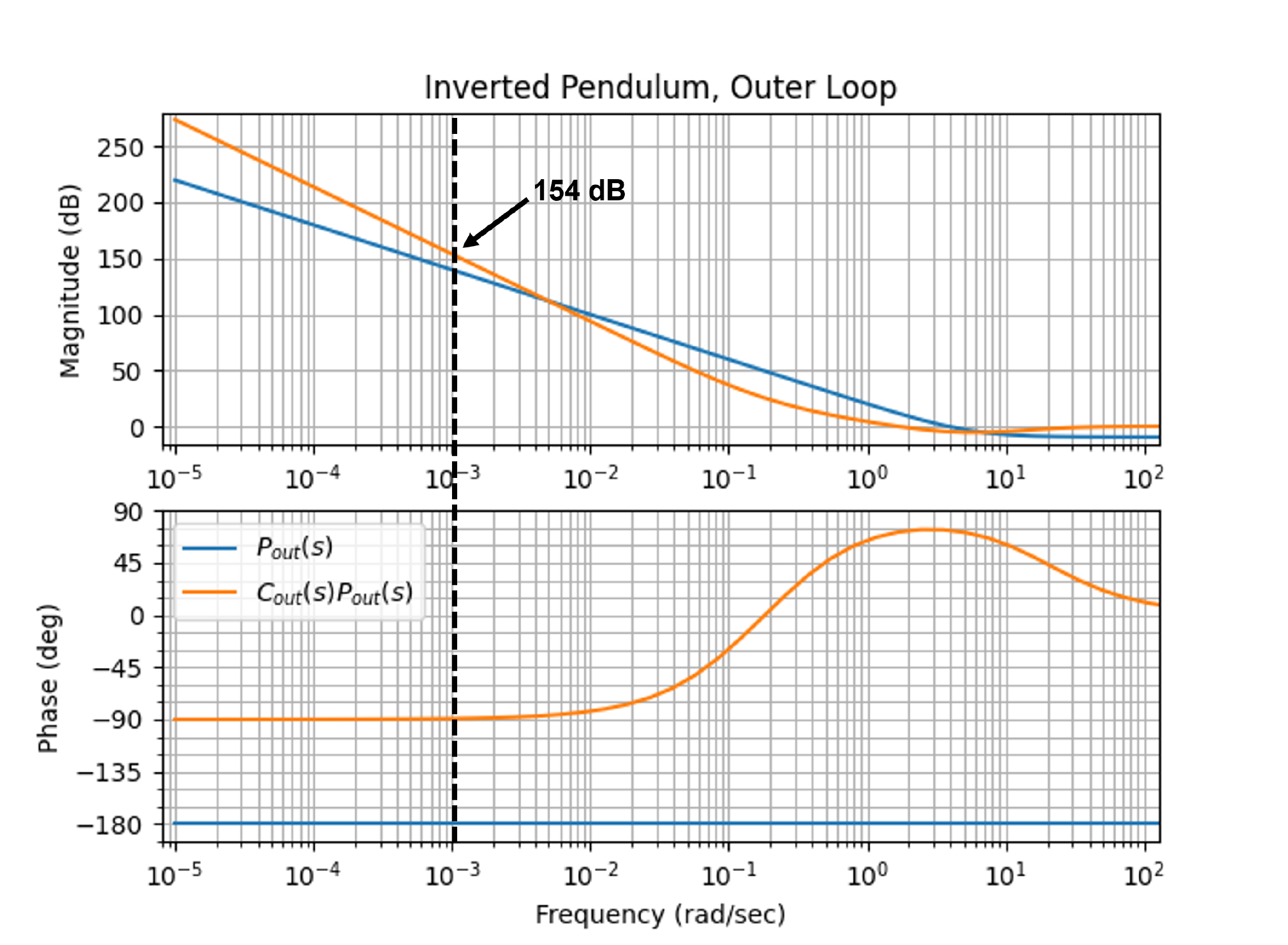
(c) The Bode plots of the outer-loop plant \(P(s)\) and the loop gain with PID control
\(P(s)C_{PID}(s)\) are shown in
Fig.16.11.
Figure 16.11. Bode plot for the outer loop of the
inverted pendulum for (1) plant only (blue), and (2) under PID control
(orange).
From Fig.16.11 it can be seen
that the loop gain under PID control for the outer loop is above \(B_r=154\) dB for all \(\omega<\omega_r=0.001\) radians/second.
Therefore, from Equation 16.5 the
tracking error satisfies \[\left|e(t)\right|\leq \gamma_r
\left|r(t)\right|,\] where \(\gamma_r =
10^{-154/20}=2.0e-08\). Therefore, if \(\left|r(t)\right|\leq 50\), then \(\left|e(t)\right|\leq 100e-08\).
For the inner loop of the satellite attitude control, use the
bode command to create a graph that simultaneously displays
the Bode plots for (1) the plant, and (2) the plant under PD control,
using the control gains calculated in
Homework 3.3.13.
(a) To what percent error can the closed-loop system under PD control track
a step in \(\theta_r(t)=20 t^2\) for
\(t\geq0\)?
(b) If the input disturbance has frequency content below \(\omega_{d_{in}}=0.1\) radians per second,
what percentage of the input disturbance appears in the output?
For the outer loop of the satellite attitude control, use the
bode command to create a graph that simultaneously displays
the Bode plots for (1) the plant, (2) the plant under PID control using
the control gains calculated in
Homework 3.3.13.
(c) If all of the frequency content of the noise \(n(t)\) is greater than \(\omega_{no} = 10\) radians per second, what
percentage of the noise shows up in the output signal \(\phi\), using PI control?
Design Study C guided exercise
Read satellite frequency-domain specs
Use Bode-plot
offsets to estimate tracking error, disturbance rejection, and noise
transmission.
Step 1. Inner-loop tracking
type
Show solution for Step
1
Answer: The inner loop is type 2
for tracking, so parabolic inputs have finite steady-state
error.
Step 2. Disturbance
frequency
Show solution for Step
2
Answer: Evaluate
input-disturbance rejection below \(\omega_{d_{in}}=0.1\) rad/s using the
dB separation between loop gain and plant.
Step 3. Outer-loop noise
Show
solution for Step 3
Answer: Noise
above \(10\) rad/s is evaluated from the high-frequency loop behavior;
reducing it trades against bandwidth and response
speed.
Complete solution
(a)
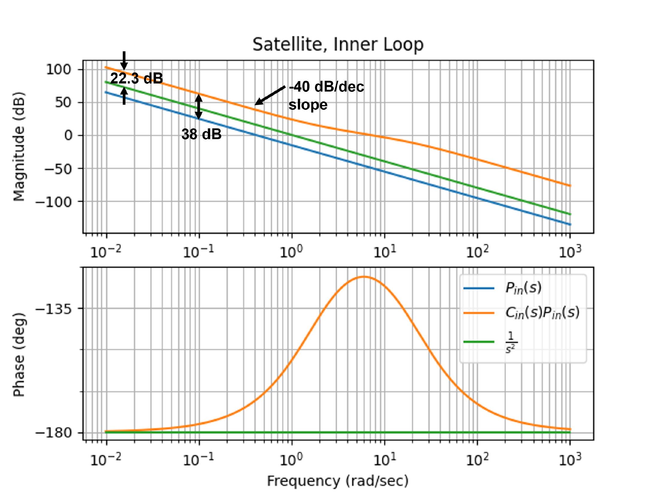
The Bode plots of the plant \(P(s)\)
and the loop gain with PD control \(P(s)C_{PD}(s)\) are shown in
Fig.16.12.
Figure 16.12. Bode plot for the inner loop of the
satellite attitude control for (a) plant only (blue), and (b) under PD
control (orange).
Suppose that the desired reference input is \(\theta^r(t) = 20t^2\). Under PD control,
the slope of the loop gain as \(\omega\to
0\) is \(-40\) dB/dec, which
implies that the system is type 2 and will track a step and a ramp with
zero steady-state error. For a parabola, there will be a finite error.
Since the loop gain under PID control is \(B_2=20\) dB above the \(1/s^2\) line, from Equation 16.12
the steady-state error satisfies \[\lim_{t\to\infty}\left|e(t)\right| \leq
\frac{A}{M_a} = 20\cdot 10^{-22.3/20} = 1.53.\]
(b) If the input disturbance is below \(\omega_{d_{in}} = 0.1\) rad/s, then the
difference between the loop gain and the plant is \(B_{d_{in}}=38\) dB, therefore, from
Equation 16.9
we see that \[\gamma_{d_{in}} = 10^{-38/20} =
0.0126,\] implying that 1.26% of the input disturbance will show
up in the output.
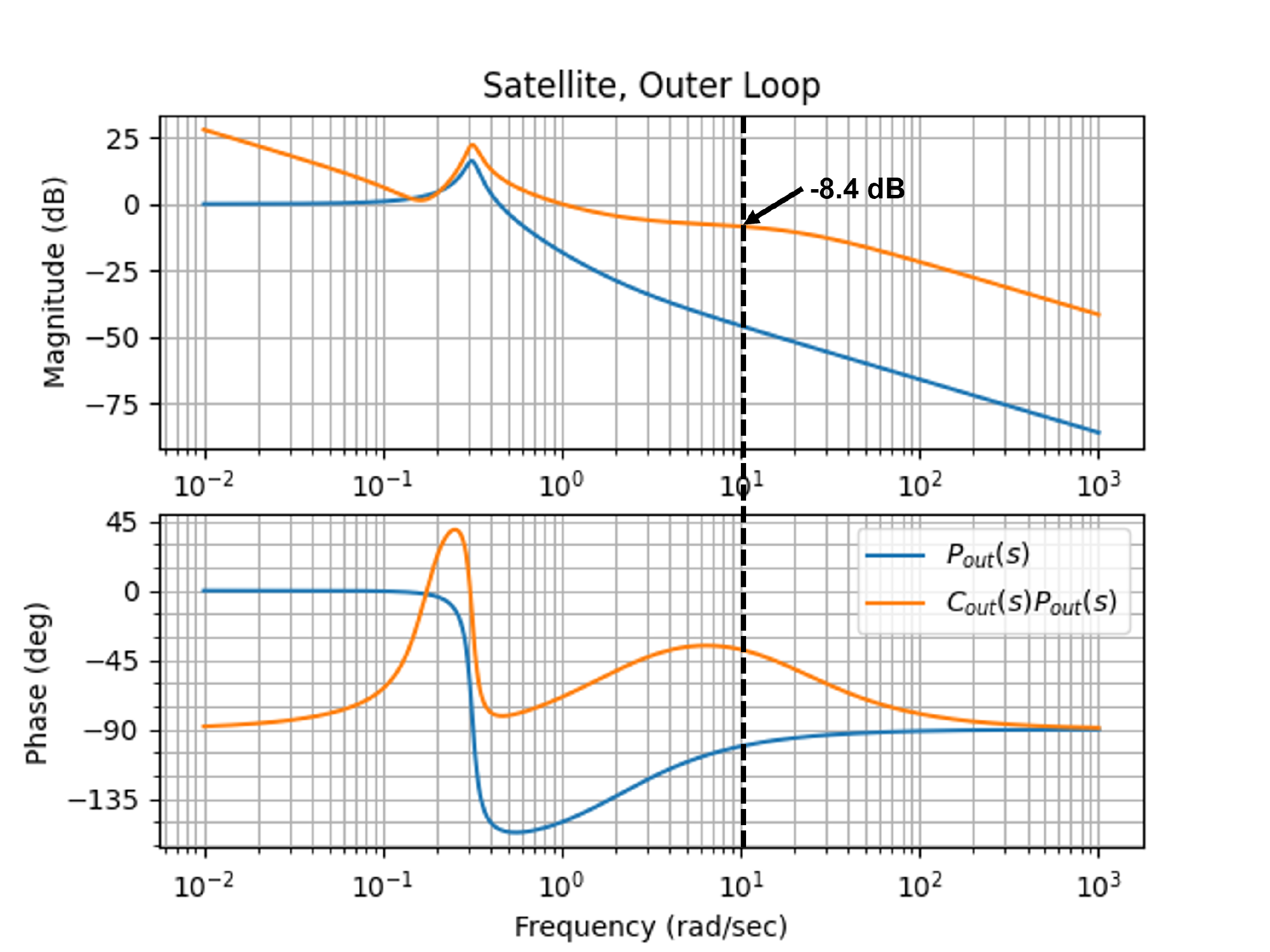
(c) The Bode plots of the outer-loop plant \(P_{out}(s)\) and the loop gain with PI
control \(P_{out}(s)C_{PI}(s)\) are
shown in Fig.16.13.
Figure 16.13. Bode plot for the outer loop of the
satellite attitude control for (a) plant only (blue), and (b) PI control
(orange).
For noise greater than \(\omega_{no}=10\) rad/sec, we see from
Fig.16.13 that \(B_n = 8.4\) dB. Therefore, \(\gamma_n = 10^{-8.4/20} = 0.380\) which
implies that \(38\)% of the noise will
show up in the output signal.
Select a specification, choose a base plant, then set the specification
frequency and dB level. The shaded region marks the acceptable part of
the loop-gain plot for that frequency-domain requirement.
The amplitude
A scales the steady-state error
calculation for the system-type cases. It does not move the Bode curves;
it changes the computed error for step, ramp, and parabolic reference
inputs.
Figure 1.8. The gray curve is the base plant magnitude |P(jω)|. The blue
curve is the loop gain |P(jω)C(jω)|
after the loop-height offset is applied.
Measured specification
At the selected
frequency:
Computed bound:
Interpretation:
16.6 Knowledge Check
Q1.
Low-frequency gain
Tracking error is
small when low-frequency loop gain is:
Q2. Noise
attenuation
Noise attenuation
generally requires loop gain to be:
Q3. Sensitivity bound
If a specification requires |S| <= 0.1, enter that bound in dB.
Show solution
Answer: -20 dB because 20 log10(0.1) = -20.
Q4. Loop-gain requirement
Approximately how many dB of loop gain are needed for |S| near 0.1
when L is large?
Show solution
Answer: About 20 dB. When L is large, S is
approximately 1/L.
Q5. Output disturbance function
Which closed-loop function is most directly associated with output
disturbance rejection?
Show solution
Answer: Sensitivity, S = 1/(1+PC), is the key function
for output disturbance and tracking error.
Q6. Noise attenuation bound
If high-frequency sensor noise should contribute
less than 1 percent to the output, what magnitude bound should the
relevant noise transfer path satisfy?
Q7. Tracking-error
function
Which closed-loop function is
most directly used to bound low-frequency reference tracking error in
unity feedback?
Q8. Disturbance location
Why do input-disturbance and output-disturbance
specifications use different transfer paths?
Q9. System type from slope
What low-frequency loop-gain slope indicates one
free integrator?
Q10. Why not high gain
everywhere?
Why not simply make the
loop gain very large at every frequency?