In the previous chapter we explored design techniques for second-order systems where the feedback controller was a PD-type control. Since second-order systems have two degrees of freedom, their transient response can be completely determined by the proportional and derivative gains. However, from the simulation results it can easily be observed that if there is a disturbance on the system, or if the controller does not know the system parameters exactly, then there will be a steady-state error in the output. The steady-state error can be effectively removed using an integrator in the control law. In this chapter we will explore these ideas in more detail and explain when and how integral control can be used to enhance steady-state tracking and to reduce the effect of disturbances.
The key theoretical tool to understanding the steady-state error and the effect of integrators is the final value theorem, which we state and prove below.
.
Suppose that \(z(t)\) and \(Z(s)\) are Laplace transform pairs, and
suppose that \(\lim_{t\to\infty}z(t)\)
is finite, then \[\lim_{t\to\infty}z(t) =
\lim_{s\to 0} sZ(s).\]
Interactive check
The final value theorem is useful only when the final value exists. Select a transform, predict whether the theorem applies, and then check the poles of sY(s).
For Y(s) = 3 / (s(s + 4)), enter the final value if the final value theorem applies.
Answer: 0.75. Since sY(s) = 3/(s + 4), the pole is at s = -4 and the theorem applies; lims->0 3/(s + 4) = 3/4.
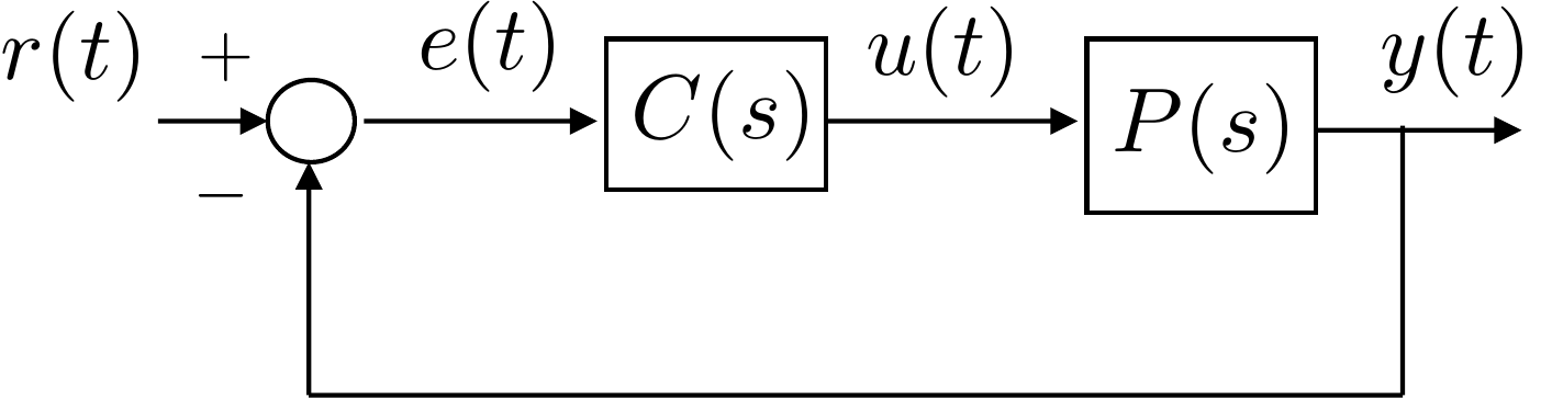
Consider the closed-loop system shown in Fig. 9.1. The transfer function from the reference \(r\) to the error \(e=r-y\) is computed as \[\begin{aligned} & E(s) = R(s) - P(s)C(s)E(s) \\ \implies & E(s) = \frac{1}{1+P(s)C(s)}R(s) \end{aligned}\]
Suppose that \(r(t)\) is a step of size one, then \(R(s)=\frac{1}{s}\) and \[E(s) = \frac{1}{1+P(s)C(s)}\frac{1}{s}.\] Assuming that the closed-loop system is stable and therefore that \(\lim_{t\to\infty}e(t)\) is finite, then the final value theorem gives \[\begin{aligned} \lim_{t\to\infty}e(t) &= \lim_{s\to 0} sE(s) \\ &= \lim_{s\to 0} s\frac{1}{1+P(s)C(s)}\frac{1}{s} \\ &= \lim_{s\to 0}\frac{1}{1+P(s)C(s)} \\ &= \frac{1}{1+\lim_{s\to 0} P(s)C(s)}. \end{aligned}\] Let \[M_p \stackrel{\triangle}{=}\lim_{s\to 0} P(s)C(s),\] then \[\lim_{t\to\infty}e(t) = \frac{1}{1+M_p}.\]
Now suppose that \[P(s)C(s) = \frac{K(s+z_1)(s+z_2)\cdots(s+z_m)}{(s+p_1)(s+p_2)\cdots(s+p_n)},\] then \[M_p = \lim_{s\to 0} P(s)C(s) = \frac{Kz_1z_2\cdots z_m}{p_1p_2\cdots p_n}.\] In this case, the steady-state error is \(\frac{1}{1+M_p}\) which is finite. Note also that the DC gain of the closed-loop system is \[k_{DC} = \frac{1}{1+M_p}.\]
Now suppose that \(P(s)C(s)\) contains a pole at the origin, or in other words, one free integrator, i.e., \[P(s)C(s) = \frac{K(s+z_1)(s+z_2)\cdots(s+z_m)}{s(s+p_1)(s+p_2)\cdots(s+p_n)}.\] In this case we have \[M_p = \lim_{s\to 0} P(s)C(s) = \infty,\] and the steady-state error is \[\lim_{t\to\infty}e(t) = \frac{1}{1+\infty} = 0.\] Therefore, one free integrator in \(P(s)C(s)\) implies that the steady-state error to a step is zero. Note that multiple free integrators, i.e., \[P(s)C(s) = \frac{K(s+z_1)(s+z_2)\cdots(s+z_m)}{s^q(s+p_1)(s+p_2)\cdots(s+p_n)},\] gives that same result for \(q\geq 1\).
Now suppose that \(r(t)\) is a unit ramp, or in other words that \(R(s)=\frac{1}{s^2}\). In this case the error is given by \[E(s) = \frac{1}{1+P(s)C(s)}\frac{1}{s^2}.\] Again assuming that the closed-loop system is stable, the final value theorem gives \[\begin{aligned} \lim_{t\to\infty} e(t) &= \lim_{s\to 0} sE(s) \\ &= \lim_{s\to 0} s \frac{1}{1+P(s)C(s)}\frac{1}{s^2} \\ &= \lim_{s\to 0} \frac{1}{s+sP(s)C(s)} \\ &= \frac{1}{\lim_{s\to 0} sP(s)C(s)}. \end{aligned}\] Defining \[M_v = \lim_{s\to 0} sP(s)C(s),\] gives \[\lim_{t\to\infty} e(t) = \frac{1}{M_v}.\] If \(P(s)C(s)\) has no free integrators, i.e., \[P(s)C(s) = \frac{K(s+z_1)(s+z_2)\cdots(s+z_m)}{(s+p_1)(s+p_2)\cdots(s+p_n)}\] then \[M_v = \lim_{s\to 0} s\frac{K(s+z_1)(s+z_2)\cdots(s+z_m)}{(s+p_1)(s+p_2)\cdots(s+p_n)} = 0.\] Therefore \[\lim_{t\to\infty} e(t) = \frac{1}{0}=\infty.\] If, on the other hand, \(P(s)C(s)\) has one free integrator, i.e., \[P(s)C(s) = \frac{K(s+z_1)(s+z_2)\cdots(s+z_m)}{s(s+p_1)(s+p_2)\cdots(s+p_n)}\] then \[M_v = \lim_{s\to 0} s \frac{K(s+z_1)(s+z_2)\cdots(s+z_m)}{s(s+p_1)(s+p_2)\cdots(s+p_n)} = \frac{Kz_1z_2\cdots z_m}{p_1p_2\cdots p_n},\] therefore the steady-state error is finite. If \(P(s)C(s)\) has two or more free integrators, then \[M_v = \lim_{s\to 0} s \frac{K(s+z_1)(s+z_2)\cdots(s+z_m)}{s^q(s+p_1)(s+p_2)\cdots(s+p_n)} = \infty,\] when \(q\geq 2\), therefore \[\lim_{t\to\infty} e(t) = \frac{1}{\infty} = 0.\] Therefore, the number of free integrators in \(P(s)C(s)\) is the key parameter for reference tracking with zero steady-state error.
For the reference tracking problem, we say that the system is type \(q\) if the steady-state error to input \(R(s) = \frac{1}{s^{q+1}}\) is finite and if the steady-state error to input \(R(s)=\frac{1}{s^p}\) is zero for \(1\leq p\leq q\). In general, for the feedback system shown in Fig. 9.1, the steady-state tracking error when \(R(s)=\frac{1}{s^{q+1}}\) is given by \[\lim_{t\to\infty}e(t) = \lim_{s\to 0} s E(s) = \lim_{s\to 0} \left(\frac{1}{1+P(s)C(s)}\right)\left(\frac{1}{s^q}\right).\] Table 12.1 summarizes the tracking error for different inputs as a function of system type, where \[\begin{aligned} M_p &= \lim_{s\to 0}P(s)C(s) \\ M_v &= \lim_{s\to 0}sP(s)C(s) \\ M_a &= \lim_{s\to 0}s^2P(s)C(s). \end{aligned}\]
| System Type | Step (\(\frac{1}{s}\)) | Ramp (\(\frac{1}{s^2}\)) | Parabola (\(\frac{1}{s^3}\)) | \(\cdots\) |
|---|---|---|---|---|
| \(0\) | \(\frac{1}{1+M_p}\) | \(\infty\) | \(\infty\) | \(\cdots\) |
| \(1\) | \(0\) | \(\frac{1}{M_v}\) | \(\infty\) | \(\cdots\) |
| \(2\) | \(0\) | \(0\) | \(\frac{1}{M_a}\) | \(\cdots\) |
| \(3\) | \(0\) | \(0\) | \(0\) | \(\cdots\) |
| \(\vdots\) | \(\vdots\) | \(\vdots\) | \(\vdots\) |
Reference tracking verse system type.
Interactive figure
Use the controls to connect the table to a visual prediction. The input order is determined by R(s), while the tracking type is determined by the number of free integrators in P(s)C(s).
Why
Error constant effect
As an example, consider the feedback system shown in Fig. 9.2.
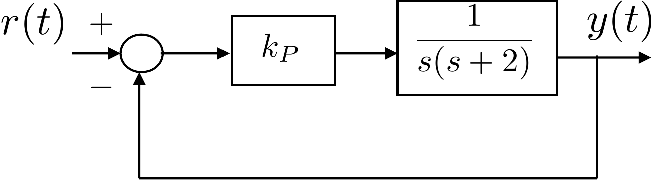
The open-loop system \[P(s)C(s) = \frac{k_P}{s(s+2)}\] has one free integrator (pole at zero) and therefore the system is type 1. From Table 12.1 the tracking error when the input is a step is zero, and the tracking error when the input is a ramp of slope one is \[\lim_{t\to\infty}e(t) = \frac{1}{M_v} = \frac{1}{\lim_{s\to 0} sP(s)C(s)} = \frac{1}{\frac{k_P}{2}} = \frac{2}{k_P}.\] The tracking error when the input is a parabola, or higher-order polynomial, is \(\infty\), meaning that \(y(t)\) and \(r(t)\) diverge as \(t\to\infty\).
As another example, consider the system shown in Fig. 9.3.
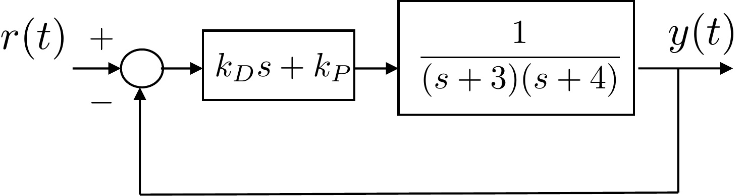
In this case, the open-loop system \[P(s)C(s) = \frac{k_D s + k_P}{(s+3)(s+4)}\] does not have any free integrators (poles at zero) and therefore the system is type 0. From Table 12.1 the tracking error when the input is a step is \[\lim_{t\to\infty}e(t) = \frac{1}{1+M_p} = \frac{1}{1+\lim_{s\to 0} P(s)C(s)} = \frac{1}{1+\frac{k_P}{12}} = \frac{12}{12+k_P}.\] The tracking error when the input is a ramp, or higher-order polynomial, is \(\infty\), meaning that \(y(t)\) and \(r(t)\) diverge as \(t\to\infty\).
If, on the other hand, a PID controller is used as shown in Fig. 9.4 where \[U(s) = \left(k_P + \frac{k_I}{s} + k_D s\right)E(s) = \left(\frac{k_D s^2 + k_P s + k_I}{s}\right)E(s),\]
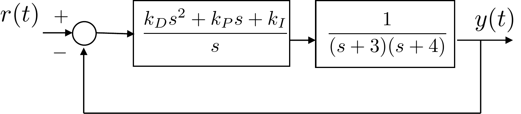
then the open-loop system \[P(s)C(s) = \frac{k_D s^2 + k_Ps + k_I}{s(s+3)(s+4)}\] has one free integrator (pole at zero) and therefore the system becomes type 1 by design. From Table 12.1 the tracking error when the input is a step is zero, and the tracking error when the input is a ramp is \[\lim_{t\to\infty}e(t) = \frac{1}{M_v} = \frac{1}{\lim_{s\to 0} sP(s)C(s)} = \frac{1}{\frac{k_I}{12}} = \frac{12}{k_I}.\] The tracking error when the input is a parabola, or higher-order polynomial, is \(\infty\), meaning that \(y(t)\) and \(r(t)\) diverge as \(t\to\infty\).
Consider the general feedback loop shown in Fig. 9.5. There are in general four inputs to the system, namely the reference input \(r(t)\), the input disturbance \(d_{in}(t)\), the output disturbance \(d_{out}(t)\), and the sensor noise \(n(t)\). In general \(r(t)\), \(d_{in}(t)\), and \(d_{out}(t)\) are signals with low frequency content, and the sensor noise \(n(t)\) has high frequency content. The negative sign on the disturbance and noise terms is for notational convenience.
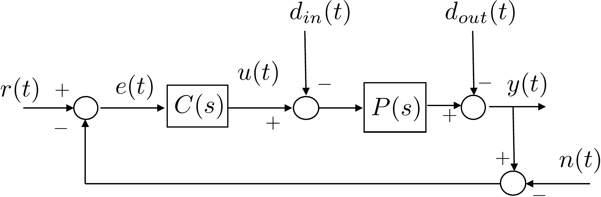
We can compute the transfer function from each input to the error signal by following the signal flow to obtain \[E(s) = R(s) + N(s) + D_{out}(s) + P(s)D_{in}(s) - P(s)C(s)E(s).\] Solving for \(E(s)\) gives \[\begin{gathered} E(s) = \frac{1}{1+P(s)C(s)} R(s) + \frac{1}{1+P(s)C(s)}N(s) \\ + \frac{1}{1+P(s)C(s)}D_{out}(s) + \frac{P(s)}{1+P(s)C(s)}D_{in}(s). \end{gathered}\] Since the transfer function from \(N(s)\) and \(D_{out}(s)\) to \(E(s)\) is identical to the transfer function from \(R(s)\) to \(E(s)\), the system type as defined in the previous section for reference inputs, also characterizes the steady-state response to output disturbances and noise. However, the transfer function from the input disturbance to the error is different, and so we need to further analyze system type with respect to input disturbances.
Suppose that the input disturbance is given by \(D_{in}(s) = \frac{1}{s^{q+1}}\), then by the final value theorem, the steady-state error due to the input disturbance is \[\lim_{t\to\infty} e(t) = \lim_{s\to 0} s\frac{P(s)}{1+P(s)C(s)}D_{in}(s) = \lim_{s\to 0} \left(\frac{P(s)}{1+P(s)C(s)}\right)\left(\frac{1}{s^q}\right).\] The system type with respect to input disturbance is the value of \(q\) such that the steady-state error is finite, and the steady-state error is zero for \(D_{in}(s) = \frac{1}{s^p}\) for \(1\leq p \leq q\).
For example, consider the system shown in Fig. 9.6. Recall from the discussion above, that the system type with respect to the reference input is type 1.
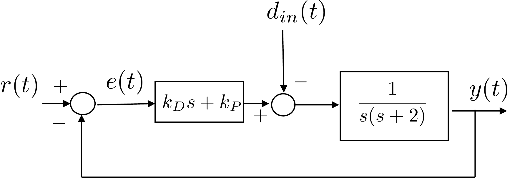
For the input disturbance we have \[\begin{aligned} \lim_{t\to\infty} e(t) &= \lim_{s\to 0} \left(\frac{P(s)}{1+P(s)C(s)}\right)\left(\frac{1}{s^q}\right) \\ &=\lim_{s\to 0} \left(\frac{\frac{1}{s(s+2)}}{1+\left(\frac{1}{s(s+2)}\right)(k_Ds+k_P)}\right)\left(\frac{1}{s^q}\right) \\ &=\lim_{s\to 0} \left(\frac{1}{s(s+2)+(k_Ds+k_P)}\right)\left(\frac{1}{s^q}\right) \\ &=\lim_{s\to 0} \left(\frac{1}{k_P}\right)\left(\frac{1}{s^q}\right) \end{aligned}\] which is finite when \(q=0\). Therefore, the system type with respect to input disturbances is type 0 and the steady-state error to a step input disturbance is \(\frac{1}{k_P}\) whereas the steady-state error with respect to a ramp and higher-order polynomials is infinite.
If, on the other hand, we add an integrator as in Fig. 9.7, then \[\begin{aligned} \lim_{t\to\infty} e(t) &= \lim_{s\to 0} \left(\frac{P(s)}{1+P(s)C(s)}\right)\left(\frac{1}{s^q}\right) \\ &=\lim_{s\to 0} \left(\frac{\frac{1}{s(s+2)}}{1+\left(\frac{1}{s(s+2)}\right)(\frac{k_Ds^2+k_Ps+k_I}{s})}\right)\left(\frac{1}{s^q}\right) \\ &=\lim_{s\to 0} \left(\frac{s}{s^2(s+2)+(k_Ds^2+k_Ps+k_I)}\right)\left(\frac{1}{s^q}\right) \\ &=\lim_{s\to 0} \left(\frac{1}{k_I}\right)\left(\frac{1}{s^{q-1}}\right) \end{aligned}\] which is finite when \(q=1\). Therefore, the system type with respect to input disturbances is type 1 and the steady-state error to a step on the input disturbance is zero. The steady-state error with respect to a ramp on the input disturbance is \(\frac{1}{k_I}\) whereas the steady-state error with respect to a parabola and higher-order polynomials on the input disturbance is infinite.
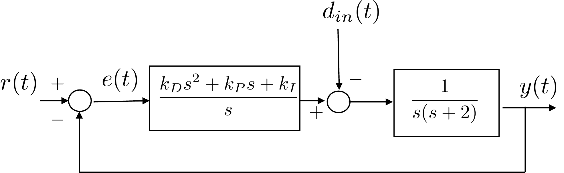
Therefore, the system type with respect to input disturbances is related to the number of free integrators in the controller \(C(s)\) and not in the open-loop system \(P(s)C(s)\). As a consequence, while an integrator may not be necessary for steady-state tracking, it is often necessary to reject constant input disturbances.
Interactive figure
Select a case to highlight where the signal enters the loop and which low-frequency path determines the steady-state error. The key distinction is that an input disturbance passes through P(s), while output disturbance and sensor noise use the same denominator path as reference tracking.
Transfer-path practice
Use the signs in the block diagram to derive the transfer functions from the external inputs R, D, and N to the error E. Do this before counting free integrators.
Which set gives the transfer functions from R, D, and N to E for the diagram above?
For the reference path E/R, which free integrators most directly increase the system type?
For the disturbance path E/D, which free integrators should you look at first?
For the low-frequency sensor-noise path E/N, which block or signal has the free integrators that most directly affect the type?
For the specific system above, enter the final
value of e(t) for each input path and polynomial input. Use
infinity for an unbounded error.
| Input path | Step | Ramp | Parabola |
|---|---|---|---|
| R to E | |||
| D to E | |||
| N to E |
Solution: The loop product is GcGpH = 1/\[s4(s+1)2\]. Therefore, E/R behaves like s4, E/D behaves like s, and E/N behaves like 2s3 near s = 0. Thus, R gives 0 for step, ramp, and parabola; D gives 0 for step, 1 for ramp, and infinity for parabola; N gives 0 for step, ramp, and parabola.
 Example Problem
3.1.12
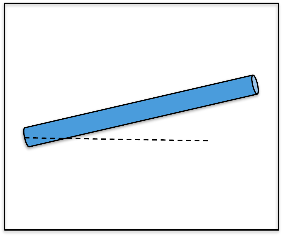
When the controller for the single-link robot arm is PD control, what is the system type? Characterize the steady-state error when the reference input is a step, a ramp, and a parabola. How does this change if you add an integrator?
Consider the case where a constant disturbance acts at the input to the plant (for example gravity in this case). What is the steady-state error to a constant input disturbance when the integrator is not present and when it is present?
Design Study A guided exercise
Count free integrators in the relevant loop transfer function before applying the final value theorem.
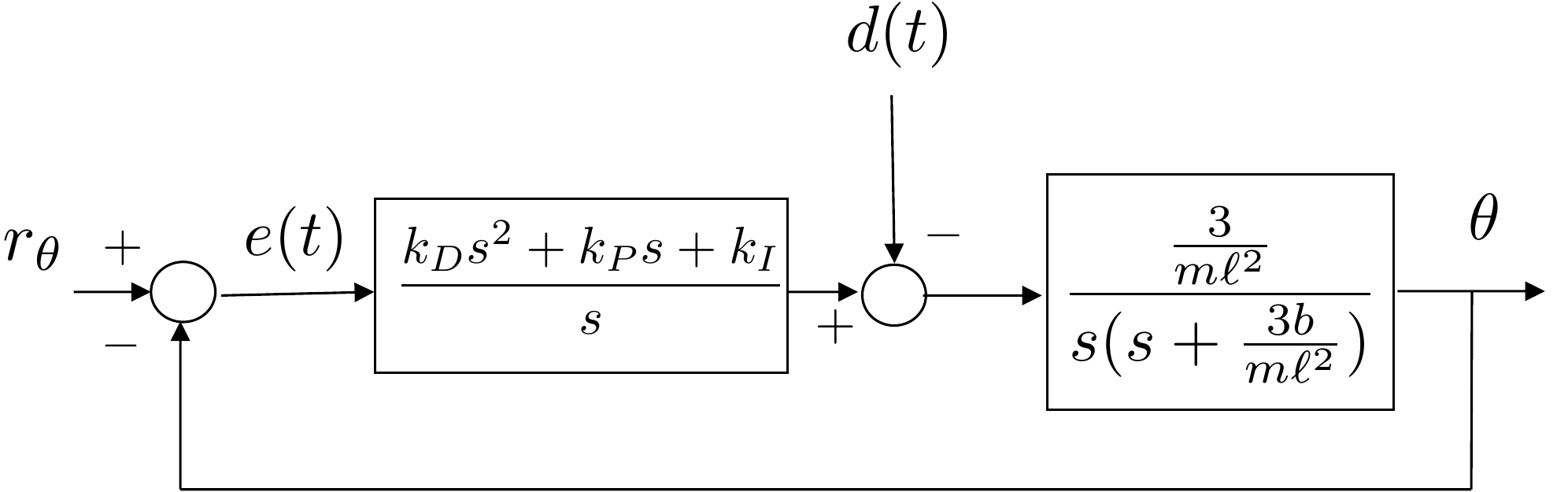
Use this closed-loop signal map to decide which loop transfer function determines tracking and disturbance error.
Answer: The arm plant contributes one free integrator, so the PD loop is type 1 for reference tracking.
Answer: Adding integral action gives two free integrators, so the reference-tracking loop is type 2.
Answer: A type 1 loop has finite ramp error; a type 2 loop has zero ramp error.
The closed-loop system is shown in Fig. 9.8.
Without the integrator, the open-loop transfer function is given by \[P(s)C(s) = \left(\frac{\frac{3}{m\ell^2}}{s(s+\frac{3b}{m\ell^2})}\right)\left(k_D s + k_P\right).\] The system has one free integrator and is therefore type 1, which, from Table 12.1 implies that the tracking error when the input is a step is zero, and the tracking error when the input is a ramp is \[\lim_{t\to\infty}e(t) = \frac{1}{M_v} = \frac{1}{\lim_{s\to 0} sP(s)C(s)} = \frac{1}{\frac{k_P}{b}} = \frac{b}{k_P}.\] The tracking error when the input is a parabola, or higher order polynomial, is \(\infty\), meaning that \(\theta(t)\) and \(\theta_r(t)\) diverge as \(t\to\infty\).
With the integrator, the open-loop transfer function is \[P(s)C(s) = \left(\frac{\frac{3}{m\ell^2}}{s(s+\frac{3b}{m\ell^2})}\right)\left(\frac{k_D s^2 + k_Ps + k_I}{s}\right).\] which has two free integrators and is therefore type 2. Therefore, from Table 12.1 the tracking error when the input is either a step or a ramp is zero, and the tracking error when the input is a parabola is \[\lim_{t\to\infty}e(t) = \frac{1}{M_a} = \frac{1}{\lim_{s\to 0} s^2P(s)C(s)} = \frac{1}{\frac{k_I}{b}} = \frac{b}{k_I}.\] The tracking error when the input is \(t^3\) or a higher order polynomial, is \(\infty\).
For the input disturbance, the transfer function from \(D(s)\) to \(E(s)\) is given by \[E(s) = \frac{P(s)}{1+P(s)C(s)}D(s).\] Without the integrator, and when \(D(s)= \frac{A}{s^{q+1}}\), the steady-state error is given by \[\begin{aligned} \lim_{t\to\infty} e(t) &= \lim_{s\to 0} \frac{P}{1+PC}\frac{A}{s^q} \\ &= \lim_{s\to 0} \left(\frac{\left(\frac{\frac{3}{m\ell^2}}{s(s+\frac{3b}{m\ell^2})}\right)}{1+\left(\frac{\frac{3}{m\ell^2}(k_Ds+k_P)}{s(s+\frac{3b}{m\ell^2})}\right)}\right)\left(\frac{A}{s^q}\right) \\ &= \lim_{s\to 0} \left(\frac{\frac{3}{m\ell^2}}{s(s+\frac{3b}{m\ell^2})+\frac{3}{m\ell^2}(k_Ds+k_P)}\right)\left(\frac{A}{s^q}\right) \\ &= \frac{A\frac{3}{m\ell^2}}{\frac{3k_P}{m\ell^2}} = \frac{A}{k_P}, \end{aligned}\] if \(q=0\). Therefore, to an input disturbance the system is type 0. The steady-state error when a constant step of size \(A\) is placed on \(d(t)\) is \(\frac{A}{k_P}\).
With the integrator, and when \(D(s)= \frac{A}{s^{q+1}}\), the steady-state error is given by \[\begin{aligned} \lim_{t\to\infty} e(t) &= \lim_{s\to 0} \frac{P}{1+PC}\frac{A}{s^q} \\ &= \lim_{s\to 0} \left(\frac{\left(\frac{\frac{3}{m\ell^2}}{s(s+\frac{3b}{m\ell^2})}\right)}{1+\left(\frac{\frac{3}{m\ell^2}}{s(s+\frac{3b}{m\ell^2})}\right)\left(\frac{k_Ds^2+k_Ps+k_I}{s}\right)}\right)\left(\frac{A}{s^q}\right) \\ &= \lim_{s\to 0} \left(s\frac{\frac{3}{m\ell^2}}{s^2(s+\frac{3b}{m\ell^2})+\frac{3}{m\ell^2}(k_Ds^2+k_Ps+k_I)}\right)\left(\frac{A}{s^q}\right) \\ &= \frac{A\frac{3}{m\ell^2}}{\frac{3k_I}{m\ell^2}} = \frac{A}{k_I}, \end{aligned}\] if \(q=1\). Therefore, to an input disturbance the system is type 1. The steady-state error when \(d(t)\) is a constant step is zero, and the steady-state error when \(d(t)\) is a ramp of slope size \(A\) is \(\frac{A}{k_I}\).
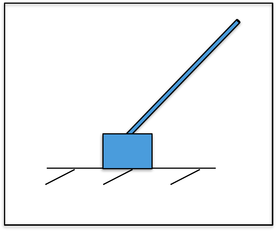 Example Problem
3.2.12
When the inner loop controller for the inverted pendulum is PD control, what is the system type with respect to tracking of the inner loop? Characterize the steady-state error when \(\tilde{R}_{\theta}\) is a step, a ramp, and a parabola. What is the system type with respect to an input disturbance?
When the outer loop controller for the inverted pendulum is PD control, what is the system type of the outer loop with respect to tracking? Characterize the steady-state error when \(r_z\) is a step, a ramp, and a parabola. How does this change if you add an integrator? What is the system type with respect to an input disturbance for both PD and PID control?
Design Study B guided exercise
Count free integrators separately for the inner and outer loops.
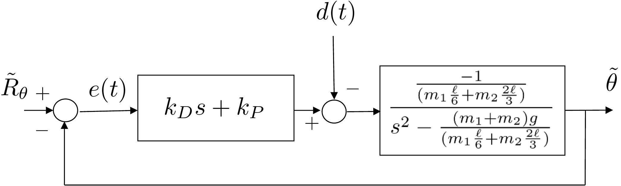
Use the inner and outer loop diagrams to decide which loop transfer function determines each steady-state error.
Answer: The inner PD loop has no free integrators for theta tracking, so it is type 0.
Answer: The outer plant contributes two free integrators, so the PD outer loop is type 2 for tracking.
Answer: Adding the integrator makes the outer tracking loop type 3.
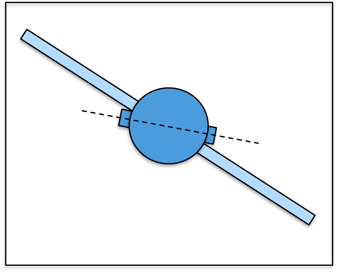
The block diagram for the inner loop is shown in Fig. 9.9.
The open-loop system is given by \[P(s)C(s) = \left(\frac{-\frac{1}{m_1\frac{\ell}{6}+m_2\frac{2\ell}{3}}}{s^2-\frac{(m_1+m_2)g}{m_1\frac{\ell}{6}+m_2\frac{2\ell}{3}}}\right)\left(k_Ds+k_P\right).\] Since there are no free integrators, the system is type 0, and from Table 12.1 the tracking error when the input is a step is \[\lim_{t\to\infty}e(t) = \frac{1}{1+M_p} = \frac{1}{1+\lim_{s\to 0} P(s)C(s)} = \frac{1}{1+\frac{k_P}{(m_1+m_2)g}}.\] The tracking error when the input is a ramp, or higher order polynomial, is \(\infty\).
For the disturbance input, the steady-state error to a step on \(d(t)\) is \[\begin{aligned} \lim_{t\to\infty}e(t) &= \lim_{s\to 0}s\frac{P(s)}{1+P(s)C(s)}\frac{1}{s} \\ &= \lim_{s\to 0} \frac{\left(\frac{-\frac{1}{m_1\frac{\ell}{6}+m_2\frac{2\ell}{3}}}{s^2-\frac{(m_1+m_2)g}{m_1\frac{\ell}{6}+m_2\frac{2\ell}{3}}}\right)}{1+\left(\frac{-\frac{1}{m_1\frac{\ell}{6}+m_2\frac{2\ell}{3}}}{s^2-\frac{(m_1+m_2)g}{m_1\frac{\ell}{6}+m_2\frac{2\ell}{3}}}\right)\left(k_Ds+k_P\right)} \\ &= \lim_{s\to 0} \frac{\left(-\frac{1}{m_1\frac{\ell}{6}+m_2\frac{2\ell}{3}}\right)}{\left(s^2-\frac{(m_1+m_2)g}{m_1\frac{\ell}{6}+m_2\frac{2\ell}{3}}\right)+\left(-\frac{1}{m_1\frac{\ell}{6}+m_2\frac{2\ell}{3}}\right)\left(k_Ds+k_P\right)} \\ &=\frac{\left(-\frac{1}{m_1\frac{\ell}{6}+m_2\frac{2\ell}{3}}\right)}{\left(-\frac{(m_1+m_2)g}{m_1\frac{\ell}{6}+m_2\frac{2\ell}{3}}\right)+\left(-\frac{k_p}{m_1\frac{\ell}{6}+m_2\frac{2\ell}{3}}\right)} = \frac{1}{(m_1+m_2)g+k_P}. \end{aligned}\] The system is type 0 with respect to the input disturbance.
The block diagram for the outer loop is shown in Fig. 9.10.
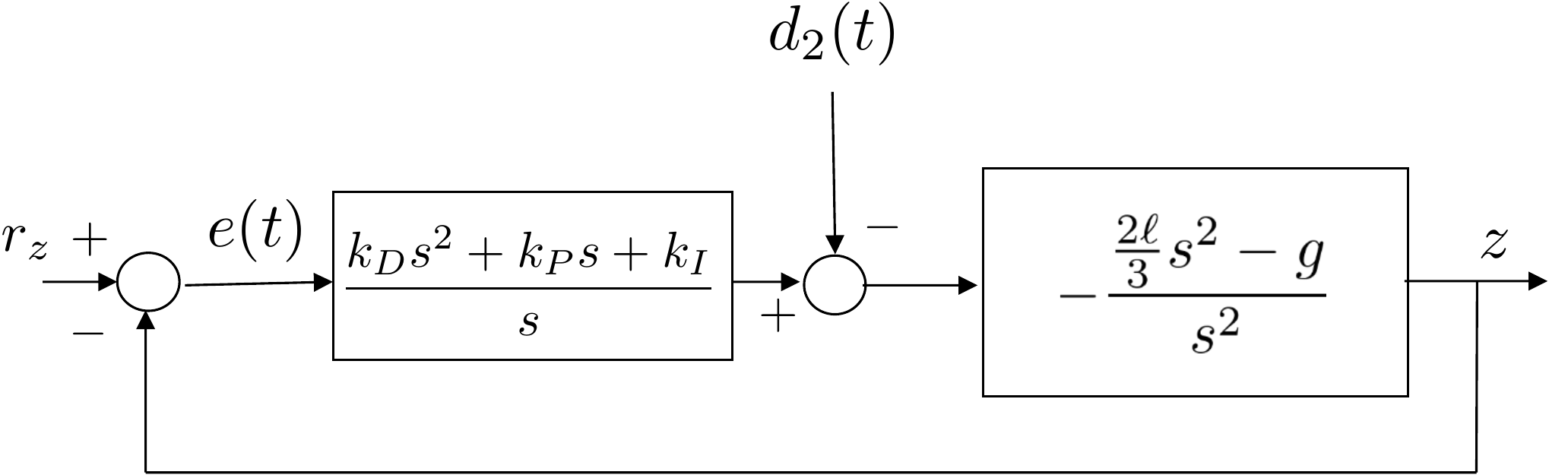
The open-loop system is given by \[P(s)C(s) = \left(\frac{\frac{-2\ell s^2}{3}+g}{s^2}\right)\left(\frac{k_Ds^2+k_Ps+k_I}{s}\right).\] When \(k_I=0\) there are two free integrators in \(P(s)C(s)\) and the system is type 2, and from Table 12.1 the tracking error when the input is a parabola is \[\lim_{t\to\infty}e(t) = \frac{1}{M_a} = \frac{1}{\lim_{s\to 0} s^2P(s)C(s)} = \frac{1}{k_Pg}.\] When \(k_I\neq 0\), there are three free integrators in \(P(s)C(s)\) and the system is type 3, with zero tracking error for a step, ramp, and parabola input.
For the disturbance input, the steady-state error when \(D(s) = \frac{1}{s^{q+1}}\) is \[\begin{aligned} \lim_{t\to\infty}e(t) &= \lim_{s\to 0}s\frac{P(s)}{1+P(s)C(s)}\frac{1}{s^{q+1}} \\ &= \lim_{s\to 0} \frac{\left(\frac{\frac{2\ell s^2}{3}-g}{s^2}\right)}{1+\left(\frac{\frac{2\ell s^2}{3}-g}{s^2}\right)\left(\frac{k_Ds^2+k_Ps+k_I}{s}\right)}\frac{1}{s^q}. \end{aligned}\] Without the integrator, i.e., when \(k_I=0\) we have \[\begin{aligned} \lim_{t\to\infty}e(t) &= \lim_{s\to 0} \frac{\frac{2\ell s^2}{3}-g}{s^2+\left(\frac{2\ell s^2}{3}-g\right)\left(k_Ds+k_P\right)}\frac{1}{s^q} = \lim_{s\to 0} \frac{g}{g\left(k_P\right)}\frac{1}{s^q} \end{aligned}\] which is finite when \(q=0\). Therefore, the system is type 0 with respect to the input disturbance and the steady-state error when \(d_2(t)\) is a unit step is \(1/k_P\).
When \(k_I\neq 0\), we have \[\begin{aligned} \lim_{t\to\infty}e(t) &= \lim_{s\to 0} \frac{s(\frac{2\ell s^2}{3}-g)}{s^3+\left(\frac{2\ell s^2}{3}-g \right)\left(k_Ds^2+k_Ps+k_I\right)}\frac{1}{s^q} = \lim_{s\to 0} \frac{g}{g\left(k_I\right)}\frac{1}{s^{q-1}} \end{aligned}\] which is finite when \(q=1\). Therefore, the system is type 1 with respect to the input disturbance and the steady-state error when \(d_2(t)\) is a unit ramp is \(1/k_I\).
 Example Problem
3.3.12
When the inner loop controller of the satellite system is PD control, what is the system type of the inner loop with respect to the reference input and with respect to the disturbance input? Characterize the steady-state error when the reference input is a step, a ramp, and a parabola. Characterize the steady-state error when the input disturbance is a step, a ramp, and a parabola.
With PD control for the outer loop, what is the system type of the outer loop with respect to the reference input and with respect to the disturbance input? Characterize the steady-state error when each of the reference and disturbance inputs is a step, a ramp, or a parabola. How does this change if you add an integrator?
Design Study C guided exercise
Separate the reference-tracking and disturbance-rejection paths for the inner and outer loops.
Answer: The inner reference path is type 2, so step and ramp reference errors are zero and parabola error is finite.
Answer: With PD outer-loop control, the outer reference path is type 0, so a step has finite nonzero error.
Answer: Adding an integrator makes the outer reference path type 1, giving zero steady-state error for a step input and finite steady-state error for a ramp input.
The block diagram for the inner loop is shown in Fig. 9.11.
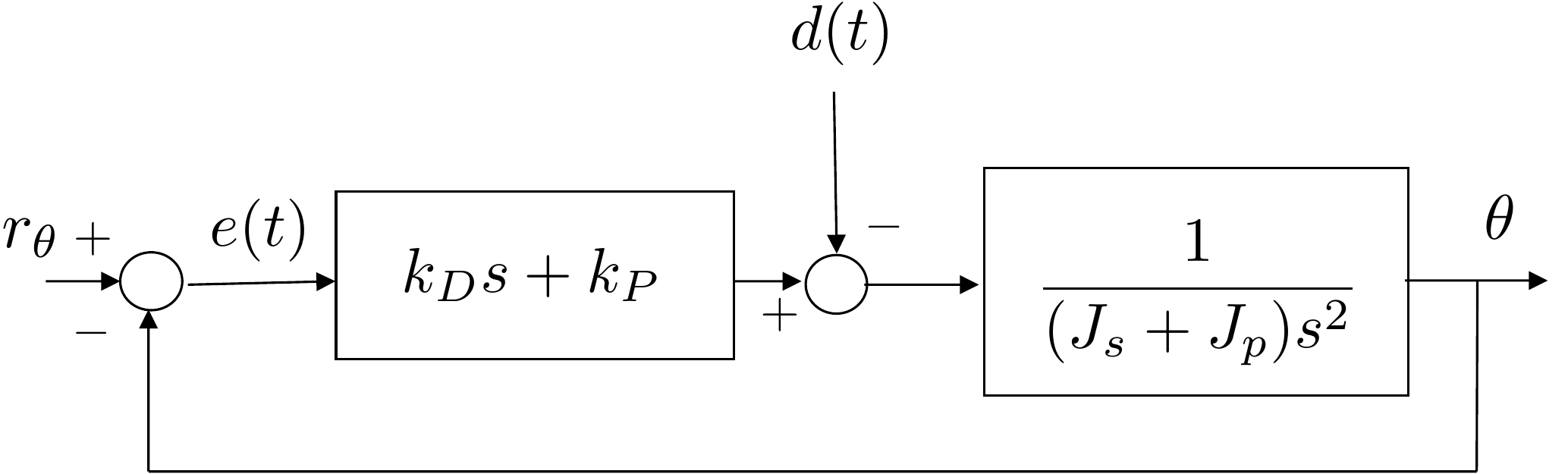
The open-loop system is given by \[% P(s)C(s) = \left(\frac{1}{(J_s + J_p)s^2}\right)\left(k_Ds+k_P\right).\] Since there are two free integrators, the system is type 2, and from Table 12.1 the tracking error when the input is a step is \[% \lim_{t\to\infty}e(t) = \frac{1}{1+M_p} = \frac{1}{1+\lim_{s\to 0} P(s)C(s)} = 0.\] The tracking error when the input is a ramp is \[\lim_{t\to\infty}e(t) = \frac{1}{M_v} = \frac{1}{\lim_{s\to 0} sP(s)C(s)} = 0.\] Finally, the tracking error when the input is a parabola is \[\lim_{t\to\infty}e(t) = \frac{1}{M_a} = \frac{1}{\lim_{s\to 0} s^2P(s)C(s)} = \frac{J_p + J_s}{k_p}.\] The tracking error for higher order polynomials is \(\infty\). For a disturbance input of \(D(s)=1/s^{q+1}\), the steady-state error is \[\begin{aligned} \lim_{t\to\infty}e(t) &= \lim_{s\to 0}s\frac{P(s)}{1+P(s)C(s)}\frac{1}{s^{q+1}} % = \lim_{s\to 0}\frac{1}{(J_s+J_p)s^2+k_ds+k_p}\frac{1}{s^q} % % \end{aligned}\] which is finite and equal to \(1/k_P\) when \(q=0\). Therefore, the system is type 0 with respect to the input disturbance, and the steady-state error to a step on \(d(t)\) is \(1/k_P\) which is infinite to a ramp and higher order polynomials.
The block diagram for the outer loop is shown in Fig. 9.12.
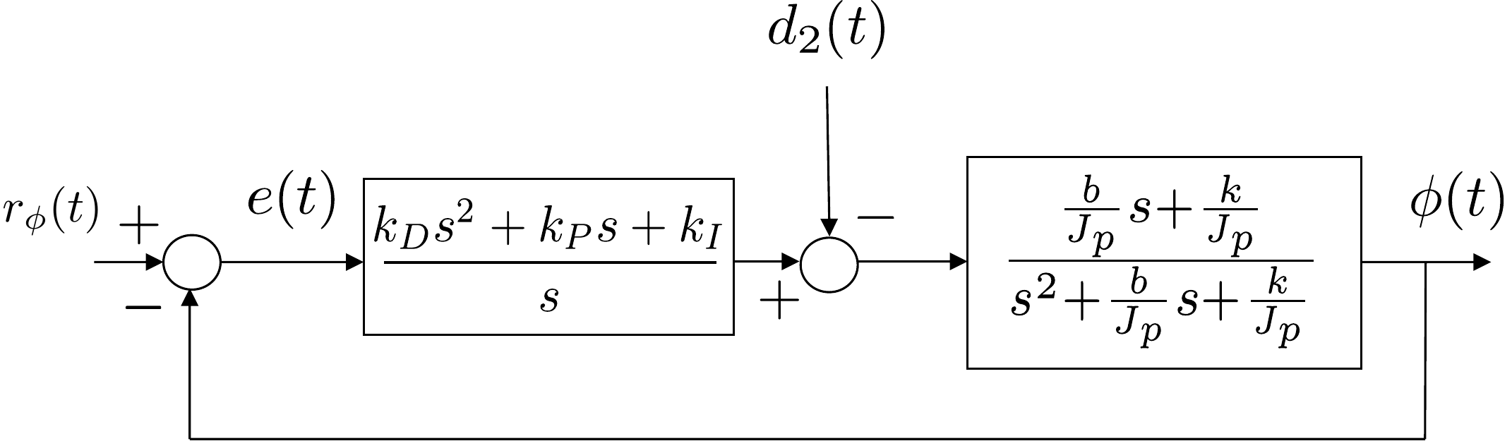
The open-loop system is given by \[P(s)C(s) = \left(\frac{\frac{b}{J_P}s+\frac{k}{J_p}}{s^2+\frac{b}{J_p}s+\frac{k}{J_p}}\right)\left(\frac{k_Ds^2+k_Ps+k_I}{s}\right).\] When \(k_I=0\) there are no free integrators in \(P(s)C(s)\) and the system is type 0, and from Table 12.1 the tracking error when the input is a step is \[\lim_{t\to\infty}e(t) = \frac{1}{1+M_p} = \frac{1}{1+\lim_{s\to 0} P(s)C(s)} = \frac{1}{1+k_P}.\] When the reference is a ramp or higher order polynomial, the tracking error is infinite. When \(k_I\neq 0\), there is one free integrator in \(P(s)C(s)\) and the system is type 1. From Table 12.1 the tracking error when the input is a ramp is \[\lim_{t\to\infty}e(t) = \frac{1}{M_v} = \frac{1}{\lim_{s\to 0} sP(s)C(s)} = \frac{1}{k_I}.\] The tracking error when \(\phi_r\) is a step is zero, and it is infinite when \(\phi_r\) is a parabola or higher order polynomial.
For the disturbance input, the steady-state error when \(D(s) = \frac{1}{s^{q+1}}\) is \[\begin{aligned} \lim_{t\to\infty}e(t) &= \lim_{s\to 0}s\frac{P(s)}{1+P(s)C(s)}\frac{1}{s^{q+1}} \\ &= \lim_{s\to 0} \frac{\left(\frac{\frac{b}{J_P}s+\frac{k}{J_p}}{s^2+\frac{b}{J_p}s+\frac{k}{J_p}}\right)}{1+\left(\frac{\frac{b}{J_P}s+\frac{k}{J_p}}{s^2+\frac{b}{J_p}s+\frac{k}{J_p}}\right)\left(\frac{k_Ds^2+k_Ps+k_I}{s}\right)}\frac{1}{s^q}. \end{aligned}\] Without the integrator, i.e., when \(k_I=0\) we have \[\begin{aligned} \lim_{t\to\infty}e(t) &= \lim_{s\to 0} \frac{\frac{b}{J_p}s+\frac{k}{J_p}}{(s^2+\frac{b}{J_p}s+\frac{k}{J_p})+(\frac{b}{J_P}s+\frac{k}{J_p})(k_Ds+k_P)}\frac{1}{s^q} \\ &= \lim_{s\to 0} \frac{1}{1+k_P}\frac{1}{s^q} \end{aligned}\] which is finite when \(q=0\). Therefore, the system is type 0 with respect to the input disturbance and the steady-state error when \(d_2(t)\) is a unit step is \(1/(1+k_P)\).
When \(k_I\neq 0\), we have \[\begin{aligned} \lim_{t\to\infty}e(t) &= \lim_{s\to 0} \frac{s\left(\frac{b}{J_p}s+\frac{k}{J_p}\right)}{s\left(s^2+\frac{b}{J_p}s+\frac{k}{J_p}\right)+\left(\frac{b}{J_p}s+\frac{k}{J_p}\right)\left(k_Ds^2+k_Ps+k_I\right)}\frac{1}{s^q} \\ &= \lim_{s\to 0} \frac{1}{k_I}\frac{1}{s^{q-1}} \end{aligned}\] which is finite when \(q=1\). Therefore, the system is type 1 with respect to the input disturbance and the steady-state error when \(d_2(t)\) is a unit ramp is \(1/k_I\). It is zero when \(d_2\) is a step, and it is infinite when \(d_2\) is a parabola or higher order polynomial.
Use these checks to test final-value theorem conditions, reference-tracking type, and disturbance-path type before moving on.
Before accepting lims->0 sY(s) as the final value, what must be true?
For reference tracking, a type 1 system has how many free integrators in P(s)C(s)?
For a stable type 1 reference-tracking system, what steady-state tracking behavior should you expect?
For input disturbances in the chapter examples, where is the free integrator that most directly improves constant disturbance rejection?
Which issue is integral action most directly intended to improve in this chapter?
A type 1 reference-tracking system has Mv = 4. For a unit ramp input, enter the steady-state error.
Answer: 0.25. For a type 1 system tracking a unit ramp, ess = 1/Mv = 1/4.
For the same type 1 reference-tracking system, enter the steady-state error for a unit step input.
Answer: 0. A type 1 system gives zero steady-state error for a step input, assuming the closed loop is stable.
If P(s)C(s) has no free integrators, enter the reference-tracking system type.
Answer: Type 0. The type equals the number of free integrators in P(s)C(s) for reference tracking.
In one word or expression, where should you look first for the free integrator that improves input-disturbance rejection in the chapter examples?
Answer: The controller C(s). For input disturbances, the chapter examples show that adding an integrator to the controller changes the disturbance type.
For unity negative feedback with plant P(s) and controller C(s), what is the transfer function from R(s) to E(s)?
For a disturbance D(s) added at the plant input in unity feedback, which closed-loop factor determines the error path magnitude from D(s) to E(s)?
For reference tracking with C(s)P(s)H(s) = 10(s + 2)/(s(s + 5)), what is the system type?
When determining the system type for a disturbance input, what should you count?
A stable type 1 reference-tracking system has Mv = 5. What is the steady-state error for a unit ramp?
The PID structure analyzed in this chapter uses a differentiator on the error as shown in Fig. 7.1 instead of differentiating the output variable as shown in Fig. 7.2. It is straightforward to show, using the final value theorem, that the system type does not change under the two configurations. However, the value of the steady-state error does change and is not necessarily given by the simple formulas in Table 12.1.