In the previous two chapters we assumed that the full state \(x\) was available to the controller for
full state feedback. In this chapter we remove that assumption and show
how the state can be reconstructed given the measurements. We will
assume that the state-space model is given by \begin{align}
\dot{x} &= Ax + Bu \tag{13.1}\\
y &= C x \tag{13.2} \\
y_r &= C_r x, \notag
\end{align} where \(y_r\in\mathbb{R}^r\) is the reference
output as discussed in the
previous two chapters, and \(y\in\mathbb{R}^p\) is the measured
output, or the signals
measured by the sensors. While the objective of the controller is to
force \(y_r(t)\) to converge to the
reference \(r(t)\), the objective of
the observer is to estimate the
state \(x(t)\) given a history of the
input \(u(t)\) and the measured output
\(y(t)\). In this book, the estimate of
the state will be denoted as \(\hat{x}(t)\).
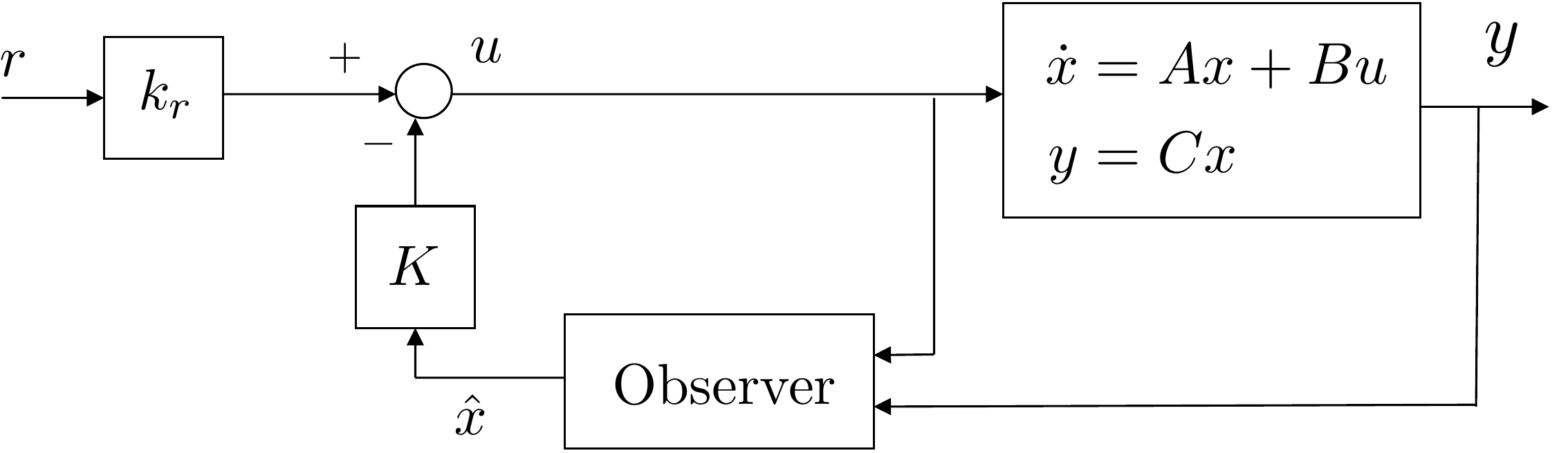
A block diagram of the closed-loop system with observer-based control
is shown in
Fig.13.1. Comparing
Fig.13.1 to the case of
full state feedback in
Fig.11.4, note that the
controller uses the estimated state \(\hat{x}\) instead of the full
state \(x\). In other words, the
controller in Equation 11.37
becomes \[u=-K\hat{x} + k_r r.\]
Figure 13.1. Closed-loop system with observer-based
feedback.
In this chapter we will design a so-called Luenberger observer that
has the structure given by \[\tag{13.3}
\dot{\hat{x}} = \underbrace{A\hat{x} + Bu}_{\text{predictor}} +
\underbrace{L \left(y - C \hat{x} \right)}_{\text{corrector}}.\]
The first term in
Equation 13.3,
i.e., \(\dot{\hat{x}}=A\hat{x}+Bu\) is
a copy of the equations of motion for the plant given in
Equation 13.1.
The second term given by \(L(y-C\hat{x})\) is a correction term, where
\(L\) is the observer gain, and \((y-C\hat{x})\) is the difference between
the measured output \(y=C x\) and the
predicted value of the measured output \(C\hat{x}\). The term \(y-C\hat{x}\) is called the
innovation signal.
Defining the observer error as \(e=x-\hat{x}\) and differentiating with
respect to time gives \[\begin{aligned}
\dot{e} &= \dot{x} - \dot{\hat{x}} \\
&= Ax + Bu - \left(A\hat{x} + Bu + Ly - LC\hat{x}\right) \\
&= A(x-\hat{x}) - LC x + LC\hat{x} \\
&= (A-LC)(x-\hat{x}) \\
&= (A-LC)e.
\end{aligned}\] Therefore, the poles that govern the
time-evolution of the observation error are given by the
eigenvalues of \(A-LC\). The observer
design problem is therefore to select \(L\) to place the eigenvalues of \(A-LC\) at locations specified by the
control engineer. The derivation of a formula for the observer gain
\(L\) proceeds in a manner similar to
the derivation of the feedback gain \(K\) in
Chapter 14.
13.1.1 Observer Design using
Observer Canonic Form
Given the general SISO monic transfer function \[\tag{13.4}
Y(s) = \frac{b_ms^m + b_{m-1}s^{m-1} + \dots + b_1 s + b_0}{s^n +
a_{n-1}s^{n-1} + \dots + a_1 s + a_0} U(s),\] where \(n>m\), and taking the inverse Laplace
transform gives \[\begin{gathered}
\frac{d^ny}{dt^n} + a_{n-1}\frac{d^{n-1}y}{dt^{n-1}} + \dots + a_1
\dot{y} + a_0 y(t)
\\ = b_m\frac{d^m u}{dt^m} + b_{m-1}\frac{d^{m-1}u}{dt^{m-1}} + \dots +
b_1 \dot{u} + b_0 u(t).
\end{gathered}\] Solving for the \(n^{th}\) derivative of \(y\) and collecting terms with similar order
derivatives gives \[\begin{gathered}
\frac{d^ny}{dt^n}
= - a_{n-1}\frac{d^{n-1}y}{dt^{n-1}} - a_{m+1}\frac{d^{m+1}y}{dt^{m+1}}
\\ + \left(b_m\frac{d^m u}{dt^m} - a_m\frac{d^m y}{dt^m}\right)
+ \dots + \left(b_1 \dot{u} - a_1 \dot{y}\right) + \left(b_0 u - a_0
y\right).
\end{gathered}\] Integrating \(n\) times gives \begin{gather}
\tag{13.5}
y(t)
= \int\Big[ - a_{n-1} y \int\Big[ - \dots - \int\Big[
- a_{m+1} y \\
+ \int\Big[\left(b_m u - a_m y\right)
+ \dots \\ + \int\Big[\left(b_1 u - a_1 y\right) + \int \left(b_0 u -
a_0 y\right) \Big]\dots\Big]\dots\Big].
\end{gather}
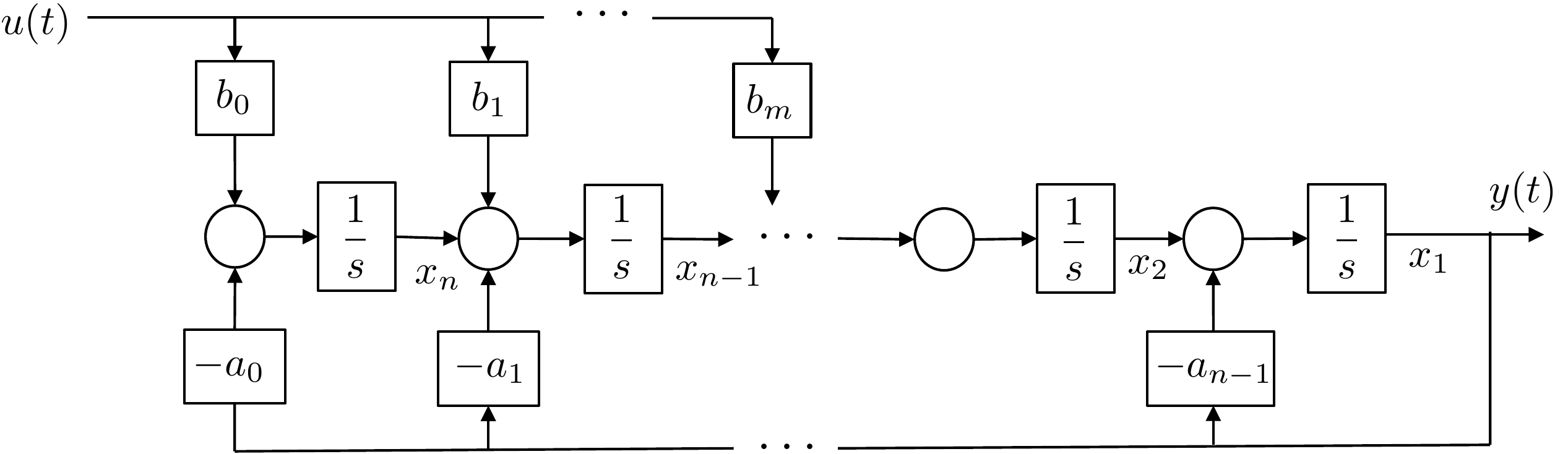
The analog computer implementation of
Equation 13.5 is shown in
Fig.13.2.
Figure 13.2. Block diagram showing the analog computer
implementation of Equation 13.5.
Labeling the states as the output of the integrators, as shown in
Fig.13.2 and
writing the equations in linear state-space form gives \begin{align}
\begin{pmatrix}\dot{x}_1 \\ \dot{x}_2 \\ \vdots \\ \dot{x}_{n-1} \\
\dot{x}_n \end{pmatrix}
&= \begin{pmatrix} -a_{n-1} & 1 & \dots & 0 & 0 \\
-a_{n-2} & 0 & \dots & 0 & 0 \\
\vdots & & \ddots & & \vdots \\
-a_1 & 0 & \dots & 0 & 1 \\
-a_0 & 0 & \dots & 0 & 0
\end{pmatrix} \begin{pmatrix} x_1 \\ x_2 \\ \vdots \\ x_{n-1} \\ x_n
\end{pmatrix}
+ \begin{pmatrix} 0 \\ \vdots \\ 0 \\ b_m \\ \vdots \\ b_1 \\ b_0
\end{pmatrix} u
\tag{13.6}\\
&y= \begin{pmatrix} 1 & 0 & \dots & 0 &
0\end{pmatrix}\begin{pmatrix} x_1 \\ x_2 \\ \vdots \\ x_{n-1} \\ x_n
\end{pmatrix}.
\tag{13.7}
\end{align} We define the observer canonic realization
as \[\begin{aligned}
\dot{x}_o &= A_o x_o + B_o u \\
y &= C_{o} x_o,
\end{aligned}\] where \begin{align}
A_o &\stackrel{\triangle}{=}\begin{pmatrix} -a_{n-1} & 1 &
\dots & 0 & 0 \\
-a_{n-2} & 0 & \dots & 0 & 0 \\
\vdots & & \ddots & & \vdots \\
-a_1 & 0 & \dots & 0 & 1 \\
-a_0 & 0 & \dots & 0 & 0
\end{pmatrix}
\tag{13.8} \\
B_o &\stackrel{\triangle}{=}\begin{pmatrix} 0 \\ \vdots \\ 0 \\ b_m
\\ \vdots \\ b_1 \\ b_0 \end{pmatrix}
\tag{13.9} \\
C_o &\stackrel{\triangle}{=}\begin{pmatrix} 1 & 0 & \dots
& 0 & 0\end{pmatrix}.
\tag{13.10}
\end{align} Comparing the state-space equations in observer
canonic form in
Equations 13.8–13.10
with the state-space equations for control canonic form in
Equations 11.14-11.16,
we see that \[\begin{aligned}
A_o &= A_c^\top \\
B_o &= C_c^\top \\
C_o &= B_c^\top.
\end{aligned}\]
Comparing the state equation in
Equation 13.6 with the
transfer function in
Equation 13.4
we see that the eigenvalues of \(A_o\)
are the roots of the open-loop characteristic polynomial \[\Delta_{ol}(s) = \det(sI-A_o) = s^n +
a_{n-1}s^{n-1} + \dots + a_1 s + a_0.\] Since \(C_o\) in
Equation 13.7 has the
structure of one in the first element followed by zeros, we see that the
structure of \(A_o-L_oC_o\) is given by
\[A_o-L_oC_o = \begin{pmatrix}
-(a_{n-1}+\ell_1) & 1 & \dots & 0 & 0 \\
-(a_{n-2}+\ell_2) & 0 & \dots & 0 & 0
\\
\vdots & & \ddots & & \vdots \\
-(a_1+\ell_{n-1}) & 0 & \dots & 0 & 1
\\
-(a_0+\ell_n) & 0 & \dots & 0 & 0
\end{pmatrix}.\] The characteristic polynomial for the
closed-loop observation error is therefore given by \[\begin{aligned}
\Delta_{cl,obs}(s) &= \det(sI-(A_o-L_oC_o)) \\
& = s^n + (a_{n-1}+\ell_1)s^{n-1} + \dots + (a_1+\ell_{n-1}) s +
(a_0+\ell_n).
\end{aligned}\] If the desired characteristic polynomial for the
closed-loop observation error is \[\tag{13.11}
\Delta_{cl,obs}^d(s) = s^n + \beta_{n-1} s^{n-1} + \dots + \beta_1 s +
\beta_0,\] then we have that \[\begin{aligned}
a_{n-1}+\ell_1 &= \beta_{n-1} \\
a_{n-2}+\ell_2 &= \beta_{n-2} \\
\vdots \\
a_1+\ell_{n-1} &= \beta_1 \\
a_0+\ell_{n} &= \beta_0.
\end{aligned}\] Defining the vectors \[\begin{aligned}
\mathbf{a}_A &\stackrel{\triangle}{=}(a_{n-1}, a_{n-2}, \dots, a_1,
a_0) \\
\boldsymbol{\beta} &\stackrel{\triangle}{=}(\beta_{n-1},
\beta_{n-2}, \dots, \beta_1, \beta_0) \\
L_o &\stackrel{\triangle}{=}(\ell_1, \ell_2, \dots, \ell_{n-1},
\ell_{n})^\top,
\end{aligned}\] we have that the observer gain satisfies \[\tag{13.12}
L_o = (\boldsymbol{\beta}-\mathbf{a}_A)^\top,\] where the
subscript “o” is used to emphasize what the gains are when the state
equations are in observer canonic form. As an example, suppose that the
transfer function model of the system is given by \[Y(s) = \frac{9s+20}{s^3+6s^2-11s+8}U(s),\]
then the state-space equations in observer canonic form are given by
\[\begin{aligned}
\dot{x}_o &= \begin{pmatrix} -6 & 1 & 0 \\ 11 & 0 &
1 \\ -8 & 0 & 0 \end{pmatrix} x_o + \begin{pmatrix} 0 \\ 9 \\ 20
\end{pmatrix} u \\
y &= \begin{pmatrix} 1 & 0 & 0 \end{pmatrix} x_o.
\end{aligned}\] The open-loop characteristic polynomial is \[\Delta_{ol}(s) = s^3+6s^2-11s+8,\] with
roots at \(-7.5885\), and \(0.7942\pm j0.6507\). Suppose that the
desired poles for the observation error are at \(-10\) and \(-20\pm j20\), then the desired closed-loop
polynomial for the observation error is \[\begin{aligned}
\Delta_{cl,obs}^d(s) &= (s+10)(s+20-j20)(s+20+j20) \\ &= s^3 +
50s^2 + 1200s + 8000,
\end{aligned}\] then \(\mathbf{a}_{A_o}=(6,-11,8)\), \(\boldsymbol{\beta}=(50,1200,8000)\), and
the observer gain that places the eigenvalues of \(A_o-L_oC_o\) at the desired locations is
given by \[L_o =
(\boldsymbol{\beta}-\mathbf{a}_{A_o})^\top = \begin{pmatrix} 50 \\ 1200
\\ 8000 \end{pmatrix} - \begin{pmatrix} 6 \\ -11 \\ 8 \end{pmatrix} =
\begin{pmatrix} 44 \\ 1211 \\ 7992 \end{pmatrix}.\]
13.1.2 Observer Design: General
State-Space Equations
The formula given in
Equation 13.12
assumes that the state-space equations are in observer canonic form.
Similar to the general full state feedback case discussed in
Section 14.1.3, a
formula for the observer gains can be derived for general state-space
equations. Following the method used in
Section 14.1.3, the
strategy is to find a state transformation matrix that converts the
general state-space equations into observer canonic form. Rather than
repeating the steps in
Section 14.1.3 we will
derive the formula for the observer gain by noting the similarities
between the design problem for full state feedback and the design
problem for the observer gain.
For full state feedback, the feedback gains \(K\) that place the eigenvalues of \(A-BK\) at the roots of the desired
characteristic equation given in
Equation 11.20
are given by
Equation 11.32
or \[\tag{13.13}
K =
(\boldsymbol{\alpha}-\mathbf{a}_A)\mathcal{A}_A^{-1}\mathcal{C}_{A,B}^{-1},\]
where \[\begin{aligned}
\mathcal{A}_A &= \begin{pmatrix}
1 & a_{n-1} & a_{n-2} & \dots & a_2 & a_1 \\
0 & 1 & a_{n-1} & \vdots & a_3 & a_2 \\
0 & 0 & 1 & \vdots & a_4 & a_3 \\
\vdots & & & \ddots & \vdots \\
0 & 0 & 0 & \dots & 1 & a_{n-1} \\
0 & 0 & 0 & \dots & 0 & 1
\end{pmatrix},
\\
\mathcal{C}_{A,B} &= \begin{pmatrix}B & AB & A^2B &
\cdots & A^{n-1}B\end{pmatrix},
\end{aligned}\] and where the subscripts are used to indicate
that \(\mathcal{A}_A\) is a function of
the matrix \(A\), and \(\mathcal{C}_{A,B}\) is a function of the
matrices \(A\) and \(B\).
The observer design problem is to find the observer gain \(L\) that places the eigenvalues of \(A-LC\) at the roots of
Equation 13.11.
Recalling from
Appendix 31 that for a general square
matrix \(M\), the eigenvalues of \(M\) equal the eigenvalues of \(M^\top\), the observer problem can be posed
as finding \(L\) that places the
eigenvalues of \(A^\top - C^\top
L^\top\) at the roots of
Equation 13.11.
This problem is identical to the full state feedback gain problem with
\(A\) replaced by \(A^\top\), \(B\) replaced by \(C^\top\), and \(K\) replaced by \(L^\top\). Making the appropriate
substitutions in Ackermann’s
formula 13.13
gives \[\tag{13.14}
L^\top =
(\boldsymbol{\beta}-\mathbf{a}_{A})\mathcal{A}_{A^\top}^{-1}\mathcal{C}_{A^\top,C^\top}^{-1}\]
Since \(\det(sI-A)=\det(sI-A^\top)\),
the characteristic equations for \(A\)
and \(A^\top\) are identical, which
implies that \(\mathbf{a}_A=\mathbf{a}_{A^\top}\) and
\(\mathcal{A}_A=\mathcal{A}_{A^\top}\).
Taking the transpose of
Equation 13.14
gives \[\tag{13.15}
L =
\mathcal{C}_{A^\top,C^\top}^{-\top}\mathcal{A}_{A}^{-\top}(\boldsymbol{\beta}-\mathbf{a}_{A})^\top,\]
where we have used the notation \[M^{-\top}\stackrel{\triangle}{=}\left(M^{-1}\right)^\top
= \left(M^\top\right)^{-1}.\] Defining the observability
matrix\[\begin{aligned}
\mathcal{O}_{A,C}
&\stackrel{\triangle}{=}\mathcal{C}_{A^\top,C^\top}^\top \\
&= \begin{pmatrix} C^\top & A^\top C^\top &
(A^\top)^2C^\top & \cdots &
(A^\top)^{n-1}C^\top\end{pmatrix}^\top \\
&= \begin{pmatrix} C \\ CA \\ CA^2 \\ \vdots \\
CA^{n-1}\end{pmatrix},
\end{aligned}\] the observer
gain 13.15
can be written as \[\tag{13.16}
L =
\mathcal{O}_{A,C}^{-1}\mathcal{A}_{A}^{-\top}(\boldsymbol{\beta}-\mathbf{a}_{A})^\top,\]
where \(L\) is well defined if the
observability matrix \(\mathcal{O}_{A,C}\) is invertible.
Accordingly, the system \((A,C)\) is
said to be observable if \(\text{rank}(\mathcal{O}_{A,C})=n\).
Equation 13.16
is Ackermann’s formula for the observer gain
\(L\). Ackermann’s formula is only
valid for single output systems. For multi-output systems there are more
advanced methods that are implemented in the MATLAB and Python
place commands. The observer gain \(L\) that places the eigenvalues of \(A-LC\) at locations \(q_1, q_2, \dots, q_n\) can be found using
the following Python commands
import numpy as np
import control as cnt

if np.linalg.matrix_rank(cnt.obsv(A,C)) != n:
    print('System Not Observable')
else:      # if so, compute observer gains
    L = cnt.place(A.T,C.T,[q1,q2,...,qn]).T
where the first operation checks to see if the system is observable
by checking whether \(\text{rank}(\mathcal{O}_{A,C})=n\). When
finding the gain \(L\) it is important
to note the three transposes which correspond to the transposes in
Equation 13.14.
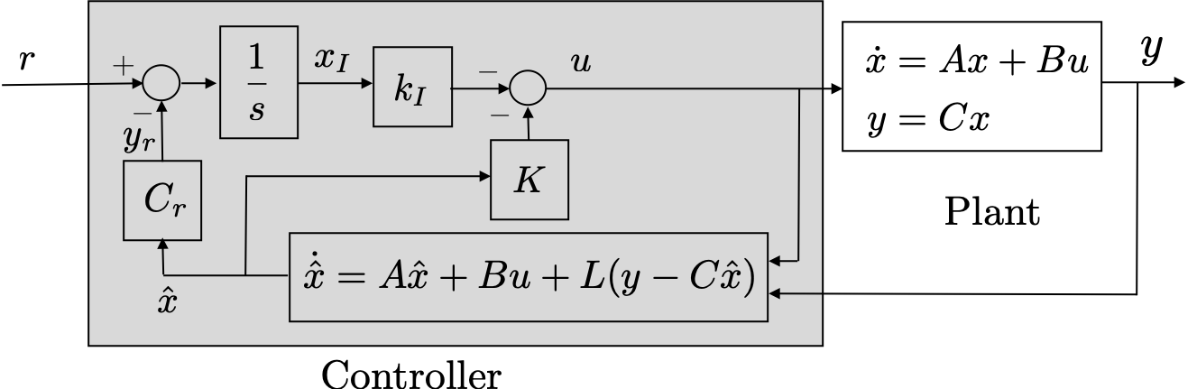
If an integrator is used in the control law, as discussed in
Chapter 15, then the
complete observer-based controller is shown in
Fig.13.3.
Note that integral feedback uses the reference
output \(y_r\), whereas the observer
uses the measured output \(y\). There
are many systems for which the measured output is identical to the
reference output.
Figure 13.3. Closed-loop system with observer-based
feedback, including integral feedback.
13.1.3 Separation Principle
The observer-based feedback design consists of two steps:
Find the state feedback gains \(K\) to place the eigenvalues of \(A-BK\) at specified locations \(p_1,\dots,p_n\),
Find the observer gains \(L\) to
place the eigenvalues of \(A-LC\) at
specified locations \(q_1,\dots,q_n\).
Since the closed-loop system includes both the observer and the state
feedback, it is important to analyze whether the closed-loop system is
stable and to determine the closed-loop poles. If the integrator is
excluded in
Fig.13.3
then the closed-loop system has \(2n\)
states: \(n\) states associated with
the open-loop plant \(x\) and \(n\) states associated with the observer
\(\hat{x}\). Since the reference input
does not affect the internal stability of the systems, we can set \(r=0\) and the equations of motion for the
closed-loop system can be written as \[\begin{aligned}
\dot{x} &= Ax + Bu \\
\dot{\hat{x}} &= A\hat{x} + Bu + L(y - C \hat{x}) \\
u &= -K\hat{x} \\
y &= C x,
\end{aligned}\] which implies that \[\begin{pmatrix} \dot{x} \\ \dot{\hat{x}}
\end{pmatrix}
= \begin{pmatrix} A & -BK \\ LC & A-BK-LC \end{pmatrix}
\begin{pmatrix} x \\ \hat{x} \end{pmatrix}.\] Recalling that a
change of variables does not change the eigenvalues of the system, and
defining the observation error as \(e=x-\hat{x}\), and noting that \[\begin{pmatrix} x \\ e \end{pmatrix} =
\begin{pmatrix} I & \mathbf{0} \\ I & -I
\end{pmatrix}\begin{pmatrix} x \\ \hat{x} \end{pmatrix},\] we
have that \[\begin{aligned}
\begin{pmatrix} \dot{x} \\ \dot{e} \end{pmatrix} &= \begin{pmatrix}
I & \mathbf{0} \\ I & -I \end{pmatrix}\begin{pmatrix} \dot{x} \\
\dot{\hat{x}} \end{pmatrix} \\
&= \begin{pmatrix} I & \mathbf{0} \\ I & -I
\end{pmatrix}\begin{pmatrix} A & -BK \\ LC & A-BK-LC
\end{pmatrix} \begin{pmatrix} x \\ \hat{x} \end{pmatrix} \\
&= \begin{pmatrix} I & \mathbf{0} \\ I & -I
\end{pmatrix}\begin{pmatrix} A & -BK \\ LC & A-BK-LC
\end{pmatrix} \begin{pmatrix} I & \mathbf{0} \\ I & -I
\end{pmatrix}^{-1} \begin{pmatrix} x \\ e \end{pmatrix},
\end{aligned}\] and noting that \[\begin{pmatrix} I & \mathbf{0} \\ I & -I
\end{pmatrix}^{-1} = \begin{pmatrix} I & \mathbf{0} \\ I & -I
\end{pmatrix}\] gives \[\begin{pmatrix} \dot{x} \\ \dot{e} \end{pmatrix}
= \begin{pmatrix} A-BK & BK \\ \mathbf{0} & A-LC \end{pmatrix}
\begin{pmatrix} x \\ e \end{pmatrix}.\] Using the determinant
properties for block diagonal matrices discussed in
Appendix 31, it is straightforward to
show that \[\text{eig}\begin{pmatrix} A-BK
& BK \\ \mathbf{0} & A-LC \end{pmatrix} = \text{eig}(A-BK)\cup
\text{eig}(A-LC).\]
Therefore, the poles of the closed-loop system are precisely the
poles selected during the design of the feedback gains \(K\) in addition to the poles selected
during the design of the observer gains \(L\). This happy circumstance is called the
separation principle, which in essence
implies that the controller and the observer can be designed separately
and then combined without affecting the stability of the system.
Unfortunately, the separation principle does not hold in general for
nonlinear systems, and even more unfortunately, while the separation
principle guarantees stability, it turns out that the addition of an
observer can negatively impact the robustness of a state feedback
design.
13.1.4 Observer Design for
Linearized Systems
Suppose that the state-space model is from a linearized system, i.e.,
suppose that \(x\in\mathbb{R}^n\) is
the state, \(x_e\in\mathbb{R}^n\) is
the equilibrium state, and that \(\tilde{x}=x-x_e\) is the state linearized
around the equilibrium. Similarly, suppose that \(u\in\mathbb{R}^m\) is the input, that \(u_e\in\mathbb{R}^m\) is the input at
equilibrium, and that \(\tilde{u}=u-u_e\) is the input linearized
around equilibrium, and that \(y\in\mathbf{R}^p\) is the measured output,
\(y_{me}=C x_e\in\mathbf{R}^p\) is the
measured output at equilibrium, and \(\tilde{y}=y-y_{e}\) is the measured output
linearized about equilibrium, then the linearized state-space model is
given by \[\begin{aligned}
\dot{\tilde{x}} &= A\tilde{x} + B\tilde{u} \\
\tilde{y} &= C\tilde{x}.
\end{aligned}\] The observer design problem then finds an
observer gain so that the eigenvalues of \(A-LC\) are at specified locations, and the
resulting observer is \[\dot{\hat{\tilde{x}}}
= A\hat{\tilde{x}} + B\tilde{u} +
L(\tilde{y}-C\hat{\tilde{x}}),\] where \(\hat{\tilde{x}}=\hat{x}-x_e\). Writing the
observer in terms of \(\hat{x}\) gives
\[\dot{\hat{x}}-\dot{x}_e = A(\hat{x}-x_e) +
B(u-u_e) + L\left((y-y_{e})-C(\hat{x}-x_e)\right).\] Noting that
\(\dot{x}_e=0\) and that \(y_{e}=C x_e\) gives \[\dot{\hat{x}} = A(\hat{x}-x_e) + B(u-u_e) +
L\left(y-C\hat{x}\right).\]
13.2 Summary of Design Process -
Observer Design
The procedure for designing an observer is summarized as follows.
Given the plant \[\begin{aligned}
\dot{x} &= Ax + Bu \\
y &= C x
\end{aligned}\] find the observer gain \(L\) so that the state observer \[\dot{\hat{x}}=A\hat{x} + Bu +
L(y-C\hat{x})\] has stable estimation error dynamics with poles
located at \(q_1, q_2, \dots,
q_n\).
Step 1.
Check to see if the system is observable by computing the observability
matrix \[\mathcal{O}_{A,C} = \begin{pmatrix}
C \\ C A \\ C A^2 \\ \vdots \\ C A^{n-1}\end{pmatrix}\] and
checking to see if \(\text{rank}(\mathcal{O}_{A,C})=n\).
Step 3.
Find the desired characteristic polynomial for the observation error
\[\begin{aligned}
\Delta_{obs}^d(s) &= (s-q_1)(s-q_2)\cdots(s-q_n) = s^n +
\beta_{n-1}s^{n-1} + \cdots + \beta_1 s + \beta_0,
\end{aligned}\] and construct the row vector \[\boldsymbol{\beta} = \begin{pmatrix}\beta_{n-1},
& \beta_{n-2}, & \dots, & \beta_1, & \beta_0
\end{pmatrix}.\]
Step 4.
Compute the desired observer gains as \[L =
\mathcal{O}_{A,C}^{-1}(\mathcal{A}_A^\top)^{-1}(\boldsymbol{\beta}-\mathbf{a}_A)^\top\]
Using Python, these steps can be implemented using the following
script.
import numpy as np
import control as cnt

if np.linalg.matrix_rank(cnt.obsv(A,C)) != n:
    print('System Not Observable')
else:   # if so, compute observer gains
    L = cnt.place(A.T,C.T,[q1,q2,...,qn]).T
13.2.1 Simple example
Given the system \[\begin{aligned}
\dot{x} &= \begin{pmatrix} 0 & 1 \\ 2 & 3 \end{pmatrix} x +
\begin{pmatrix} 0 \\ 4 \end{pmatrix} u \\
y &= \begin{pmatrix} 5 & 0 \end{pmatrix} x
\end{aligned}\] find the observer gain \(L\) so that the state observer \[\dot{\hat{x}} = A\hat{x} + Bu +
L(y-C\hat{x})\] has stable estimation error dynamics with poles
located at \(-10\pm j10\).
Step 1.
The observability matrix is given by \[\mathcal{O} = \begin{pmatrix} C \\ CA
\end{pmatrix} = \begin{pmatrix} 5 & 0 \\ 0 & 5
\end{pmatrix}.\] The determinant is \(det(\mathcal{O})=25\neq 0\), therefore the
system is observable.
Step 3.
The desired characteristic polynomial for the observation error is \[\Delta_{obs}^d(s) =
(s+10-j10)(s+10+j10)=s^2+20s+200,\] which implies that \[\boldsymbol{\beta} = \begin{pmatrix} 20, &
200 \end{pmatrix}.\]
Alternatively, we could have used the following Python script
import numpy as np
import control as cnt

# original state-space system
A = np.array([[0.0, 1.0], [2.0, 3.0]])
B = np.array([[0.0], [4.0]])
C = np.array([[5.0, 0.0]])

# desired poles for observer
q1 = -10 + 10.j
q2 = -10 - 10.j

# is the system observable?
if np.linalg.matrix_rank(cnt.obsv(A,C)) != np.size(A,1):
    print('System Not Observable')
else:  # if so, compute observer gains
    L = cnt.place(A.T,C.T,[q1,q2]).T
The corresponding observer is given by \[\tag{13.17}
\dot{\hat{x}} = \begin{pmatrix} 0 & 1 \\ 2 & 3
\end{pmatrix}\hat{x} + \begin{pmatrix} 0 \\ 4 \end{pmatrix} u +
\begin{pmatrix} 23/5 \\ 271/5 \end{pmatrix} \left( y - \begin{pmatrix} 5
& 0 \end{pmatrix}\hat{x} \right),\] and can be implemented as
member functions within a Python class as follows (see the solutions for
case studies A-C for class-specific implementation examples):
Digital implementation of the observer in
Equation 13.17 requires
two persistent (or member) variables, one for \(\hat{x}\) and one for \(u\). The observer is updated using the RK4
algorithm in lines 3–8. The differential equation that describes the
observer is given on lines 15–17.
Chapter 13 guided activity
Work through a second observer design
Use the same procedure as the simple example above. For the system
below, compute each quantity in order and click Check
before moving on. The solution for each step is revealed only after that
step is checked.
Desired observer poles: -4 ±
j3.
Step 1. Observability matrix
Compute O = (C; CA). Enter the four entries row by row and the rank.
O =
Show solution
Answer: O = (2, 0; 0, 2), so rank(O) = 2 and the system
is observable.
The objective of this problem is to design an observer that estimates
the state of the system and uses the estimated state in the controller
designed in
Homework 3.1.15.
For the sake of understanding the function of the observer, for this
problem we will use exact parameters, without an input disturbance.
Modify the arm dynamics so that the parameters known to the controller
are the actual plant parameters (uncertainty parameter \(\alpha=0\)).
Verify that the state-space system is observable by checking that
\(\text{rank}(\mathcal{O}_{A,C})=n\).
Modify the controller to add an observer to estimate the state \(\hat{x}\), and then use the estimate of the
state \(\hat{x}\) in your feedback
controller. Tune the poles of the controller and observer to obtain good
performance.
Modify the simulation files so that the controller outputs both \(u\) and \(\hat{x}\). Add a plotting routine to plot
both the state and the estimated state of the system on the same
graph.
As motivation for the next chapter, add an input disturbance to the
system of \(0.05\) and observe that
there is steady-state error in the response. This is caused by a
steady-state error in the observation error. In the next chapter we will
show how to remove the steady-state error in the observation error.
Design Study A guided exercise
Design the observer
Check observability, choose faster
observer poles, and interpret estimated states.
Step 1. Observability rank
Show solution for Step
1
Answer: The arm model is
observable from the measured angle because \(\operatorname{rank}(\mathcal{O})=2\).
Step 2. Observer pole speed
Show solution for Step
2
Answer: Observer poles are
typically placed faster than the controller poles so estimation error
decays quickly.
Step
3. Estimated state notation
Show solution for Step
3
Answer: The observer produces
\(\hat{x}\), which is used by the
controller in place of the full measured state.
Pseudocode
The complete solution includes separate
observer-update and control-update functions. Before opening it, outline
each component separately.
These prompts are ungraded. They are
intended to connect the observer equations to the implementation code in
the complete solution.
Complete solution
A Python class that implements observer-based control with an
integrator for the single link robot arm is shown below.
# 3rd-partyimport numpy as npimport control as cnt# local (controlbook)from . import params as Pfrom ..common.controller_base import ControllerBaseclass ArmSSIOController(ControllerBase):def__init__(self, separate_integrator=True):# control tuning parameters tr =0.489 zeta =0.707 integrator_pole = [-5.0]# augmented system A1 = np.block([[P.A, np.zeros((2, 1))], [-P.Cr, np.zeros(1)]]) B1 = np.vstack((P.B, 0))# check controllabilityif np.linalg.matrix_rank(cnt.ctrb(A1, B1)) !=3:raiseValueError("System not controllable")# compute control gains wn =2.2/ tr # assumes zeta = 0.707 des_char_poly = [1, 2* zeta * wn, wn**2] des_sys_poles = np.roots(des_char_poly) des_poles = np.hstack((des_sys_poles, integrator_pole))self.K1 = cnt.place(A1, B1, des_poles)self.K =self.K1[:, :2]self.ki =self.K1[:, 2:]# linearization pointself.x_eq = P.x_eqself.r_eq = P.Cr @self.x_eqself.x1_eq = np.hstack((self.x_eq, 0))# integrator variablesself.error_prev =0.0self.error_integral =0.0self.separate_integrator = separate_integrator####### OBSERVER DESIGN ######### observer tuning parameters M_obs =10.0# time scale separation between controller and observer tr_obs = tr / M_obs zeta_obs =0.707# check observabilityif np.linalg.matrix_rank(cnt.ctrb(P.A.T, P.Cm.T)) !=2:raiseValueError("System not observable")# compute observer gain matrix wn_obs =2.2/ tr_obs obs_char_poly = [1, 2* zeta_obs * wn_obs, wn_obs**2] obs_poles = np.roots(obs_char_poly)self.L = cnt.place(P.A.T, P.Cm.T, obs_poles).Tprint("L^T:", self.L.T)# observer variablesself.xhat_tilde = np.zeros(2)self.u_prev = np.zeros(1)def update_with_state(self, r, x):raiseNotImplementedError("This controller only uses measurement feedback.")def update_with_measurement(self, r, y):# update the observer with the measurement xhat =self.observer_rk4_step(y)# convert to linearization (tilde) variables x_tilde = xhat -self.x_eq# integrate error error = r - P.Cr @ xhat # can also use tilde vars (eq subtracts out)self.error_integral += P.ts * (error +self.error_prev) /2self.error_prev = error# compute feedback controlifself.separate_integrator: u_tilde =-self.K @ x_tilde -self.ki @self.error_integralelse: x1_tilde = np.hstack((x_tilde, self.error_integral)) u_tilde =-self.K1 @ x1_tilde# convert back to original variables (for feedback linearization) theta = xhat[0] u_fl = P.m * P.g * P.ell /2* np.cos(theta) u_unsat = u_tilde + u_fl u =self.saturate(u_unsat, u_max=P.tau_max)# save the previous control input for the observerself.u_prev = ureturn u, xhatdef observer_f(self, xhat_tilde, y): xhat = xhat_tilde +self.x_eq y_error = y - P.Cm @ xhat # can also use tilde vars (eq subtracts out) u_fl = P.m * P.g * P.ell /2* np.cos(xhat[0]) u_tilde =self.u_prev - u_fl xhat_tilde_dot = P.A @ xhat_tilde + P.B @ u_tilde +self.L @ y_errorreturn xhat_tilde_dotdef observer_rk4_step(self, y): k1 =self.observer_f(self.xhat_tilde, y) k2 =self.observer_f(self.xhat_tilde + P.ts /2* k1, y) k3 =self.observer_f(self.xhat_tilde + P.ts /2* k2, y) k4 =self.observer_f(self.xhat_tilde + P.ts * k3, y) xhat_tilde_dot = (k1 +2* k2 +2* k3 + k4) /6self.xhat_tilde += xhat_tilde_dot * P.ts xhat =self.xhat_tilde +self.x_eqreturn xhat
Notice that we must update the observer dynamics and that \(\hat{x}\) is used in the controller instead
of \(x\), but otherwise this controller
is identical to the controller in Chapter 15. The observer is
updated using the RK4 algorithm (see line 48). The differential
equations for the observer are also specified on lines 64–66.
Complete simulation code for MATLAB, Python, and Simulink can be
downloaded at http://controlbook.byu.edu.
The objective of this problem is to design an observer that estimates
the state of the system and to use the estimated state in the controller
designed in Homework 3.2.15.
For the sake of understanding the function of the observer, for this
problem we will use exact parameters, without an input disturbance.
Modify the pendulum dynamics so that the parameters known to the
controller are the actual plant parameters (uncertainty parameter \(\alpha=0\)).
Verify that the state-space system is observable by checking that
\(\text{rank}(\mathcal{O}_{A,C})=n\).
In the control block, add an observer to estimate the state \(\hat{x}\), and use the estimate of the
state in your feedback controller. Tune the poles of the controller and
observer to obtain good performance.
Modify the simulation files so that the controller outputs both \(u\) and \(\hat{x}\). Add a plotting routine to plot
both the state and the estimated state of the system on the same
graph.
As motivation for the next chapter, add an input disturbance to the
system of \(0.05\) and observe that
there is steady-state error in the response even though there is an
integrator. This is caused by a steady-state error in the observation
error. In the next chapter we will show how to remove the steady-state
error in the observation error.
Design
Study B guided exercise
Design the pendulum observer
Use measured z and theta to estimate the full state for
feedback.
Step 1. Observability
Show solution for
Step 1
Answer: The four-state
system must be observable from the measured outputs.
Step 2.
Observer pole choice
Show
solution for Step 2
Answer:
Observer poles are placed faster than controller poles so estimation
error decays quickly.
Step
3. Estimated state use
Show solution for Step
3
Answer: The controller uses xhat
in place of the full measured state.
Pseudocode
The complete solution includes separate
observer-update and control-update functions. Before opening it, outline
each component separately.
These prompts are ungraded. They are
intended to connect the derivation to the implementation code in the
complete solution.
Complete solution
A Python class that implements observer-based control with an
integrator for the inverted pendulum is shown below.
# 3rd-partyimport numpy as npimport control as cnt# local (controlbook)from . import params as Pfrom ..common.controller_base import ControllerBaseclass CartPendulumSSIOController(ControllerBase):def__init__(self, separate_integrator=True):# tuning parameters tr_theta =0.8# tuned for slower, more stable response.# May be necessary due to initial value for theta (10 degrees). zeta_theta =0.9 M =3 tr_z = tr_theta * M zeta_z =0.9 integrator_pole = [-2.0]# augmented system A1 = np.block([[P.A, np.zeros((4, 1))], [-P.Cr, np.zeros(1)]]) B1 = np.vstack((P.B, 0))# check controllabilityif np.linalg.matrix_rank(cnt.ctrb(A1, B1)) !=5:raiseValueError("System not controllable")# compute gains wn_theta =0.5* np.pi / (tr_theta * np.sqrt(1- zeta_theta**2)) theta_char_poly = [1, 2* zeta_theta * wn_theta, wn_theta**2] theta_poles = np.roots(theta_char_poly) wn_z =0.5* np.pi / (tr_z * np.sqrt(1- zeta_z**2)) z_char_poly = [1, 2* zeta_z * wn_z, wn_z**2] z_poles = np.roots(z_char_poly) des_poles = np.hstack([theta_poles, z_poles, integrator_pole])self.K1 = cnt.place(A1, B1, des_poles)self.K =self.K1[:, :4]self.ki =self.K1[:, 4:]# linearization pointself.x_eq = P.x_eqself.r_eq = P.Cr @self.x_eqself.u_eq = P.u_eq# integrator variablesself.error_prev =0.0self.error_integral =0.0self.separate_integrator = separate_integrator####### OBSERVER DESIGN ######### observer tuning parameters M_obs =10.0# time scale separation between controller and observer tr_theta_obs = tr_theta / M_obs zeta_theta_obs =0.9 tr_z_obs = tr_z / M_obs zeta_z_obs =0.9# check observabilityif np.linalg.matrix_rank(cnt.ctrb(P.A.T, P.Cm.T)) !=4:raiseValueError("System not observable")# compute observer gain matrix wn_theta_obs =2.2/ tr_theta_obs theta_obs_char_poly = [1, 2* zeta_theta_obs * wn_theta_obs, wn_theta_obs**2] theta_obs_poles = np.roots(theta_obs_char_poly) wn_z_obs =2.2/ tr_z_obs z_obs_char_poly = [1, 2* zeta_z_obs * wn_z_obs, wn_z_obs**2] z_obs_poles = np.roots(z_obs_char_poly) obs_poles = np.hstack((theta_obs_poles, z_obs_poles))self.L = cnt.place(P.A.T, P.Cm.T, obs_poles).Tprint("L^T:", self.L.T)# observer variablesself.xhat_tilde = np.zeros(4)self.u_prev = np.zeros(1)def update_with_state(self, r, x):raiseNotImplementedError("This controller only uses measurement feedback.")def update_with_measurement(self, r, y):# update the observer with the measurement xhat =self.observer_rk4_step(y)# convert to linearization (tilde) variables x_tilde = xhat -self.x_eq r_tilde = r -self.r_eq# integrate error error = r - P.Cr @ xhat # can also use tilde vars (eq subtracts out)self.error_integral += P.ts * (error +self.error_prev) /2self.error_prev = error# compute feedback controlifself.separate_integrator: u_tilde =-self.K @ x_tilde -self.ki @self.error_integralelse: x1_tilde = np.hstack((x_tilde, self.error_integral)) u_tilde =-self.K1 @ x1_tilde# convert back to original variables u_unsat = u_tilde +self.u_eq u =self.saturate(u_unsat, u_max=P.force_max)# save the previous control input for the observerself.u_prev = ureturn u, xhatdef observer_f(self, xhat_tilde, y): xhat = xhat_tilde +self.x_eq y_error = y - P.Cm @ xhat # can also use tilde vars (equil. terms subtract out) u_tilde =self.u_prev -self.u_eq xhat_tilde_dot = P.A @ xhat_tilde + P.B @ u_tilde +self.L @ y_errorreturn xhat_tilde_dotdef observer_rk4_step(self, y): k1 =self.observer_f(self.xhat_tilde, y) k2 =self.observer_f(self.xhat_tilde + P.ts /2* k1, y) k3 =self.observer_f(self.xhat_tilde + P.ts /2* k2, y) k4 =self.observer_f(self.xhat_tilde + P.ts * k3, y) xhat_tilde_dot = (k1 +2* k2 +2* k3 + k4) /6self.xhat_tilde += xhat_tilde_dot * P.ts xhat =self.xhat_tilde +self.x_eqreturn xhat
The observer is updated on line 25, and \(\hat{x}\) is used in the controller instead
of \(x\) but otherwise is identical to
the controller in Chapter 15. The observer is
updated on lines 40–48 using the RK4 algorithm. The differential
equations for the observer are specified on lines 50–56.
Complete simulation code for MATLAB, Python, and Simulink can be
downloaded at http://controlbook.byu.edu.
The objective of this problem is to design an observer that estimates
the state of the system and to use the estimated state in the controller
designed in Homework 3.3.15.
For the sake of understanding the function of the observer, for this
problem we will use exact parameters, without an input disturbance.
Modify the satellite dynamics so that the parameters known to the
controller are the actual plant parameters (uncertainty parameter \(\alpha=0\)).
Verify that the state-space system is observable by checking that
\(\text{rank}(\mathcal{O}_{A,C})=n\).
In the control block, add an observer to estimate the state \(\hat{x}\), and use the estimate of the
state in your feedback controller. Tune the poles of the controller and
observer to obtain good performance.
Modify the simulation files so that the controller outputs both \(u\) and \(\hat{x}\). Add a plotting routine to plot
both the state and the estimated state of the system on the same
graph.
As motivation for the next chapter, add an input disturbance to the
system of \(1.0\) Newton-meter and
observe that there is steady-state error in the response even though
there is an integrator. This is caused by a steady-state error in the
observation error. In the next chapter we will show how to remove the
steady-state error in the observation error.
Design Study C guided exercise
Plan the satellite observer
The observer estimates the
full four-state satellite state from measured outputs.
Step 1. Observer
setup
Show solution for Step
1
Answer: Use \(\alpha=0\) initially and estimate \(\hat{x}\).
Step 2.
Observability check
Show solution for
Step 2
Answer: Verify \(\operatorname{rank}(\mathcal{O}_{A,C})=n\) using
outputs \(\theta\) and \(\phi-\theta\).
Step 3. Motivation for disturbance
observers
Show solution for Step
3
Answer: Adding a 1 Nm disturbance
exposes steady-state error related to observation error, motivating
Chapter 14.
Complete solution
A Python class that implements observer-based control with an
integrator for the satellite is shown below.
# 3rd-partyimport numpy as npimport control as cnt# local (controlbook)from . import params as Pfrom ..common.controller_base import ControllerBaseclass SatelliteSSIOController(ControllerBase):def__init__(self, separate_integrator=False):# tuning parameters tr_theta =2.0 zeta_theta =0.9 M =3# time separation factor between inner and outer loop tr_phi = tr_theta * M zeta_phi =0.9 integrator_pole = [-1.0]# augmented system A1 = np.block([[P.A, np.zeros((4, 1))], [-P.Cr, np.zeros(1)]]) B1 = np.vstack((P.B, 0))# check controllabilityif np.linalg.matrix_rank(cnt.ctrb(A1, B1)) !=5:raiseValueError("System not controllable")# compute gains wn_theta =0.5* np.pi / (tr_theta * np.sqrt(1- zeta_theta**2)) theta_char_poly = [1, 2* zeta_theta * wn_theta, wn_theta**2] theta_poles = np.roots(theta_char_poly) wn_phi =0.5* np.pi / (tr_phi * np.sqrt(1- zeta_phi**2)) phi_char_poly = [1, 2* zeta_phi * wn_phi, wn_phi**2] phi_poles = np.roots(phi_char_poly) des_poles = np.hstack([theta_poles, phi_poles, integrator_pole])self.K1 = cnt.place(A1, B1, des_poles)self.K =self.K1[:, :4]self.ki =self.K1[:, 4:]# linearization pointself.x_eq = P.x_eqself.r_eq = P.Cr @self.x_eqself.u_eq = P.u_eq# integrator variablesself.error_prev =0.0self.error_integral =0.0self.separate_integrator = separate_integrator####### OBSERVER DESIGN ######### observer tuning parameters M_obs =10.0# time scale separation between controller and observer tr_theta_obs = tr_theta / M_obs zeta_theta_obs =0.9 tr_phi_obs = tr_phi / M_obs phieta_phi_obs =0.9# check observabilityif np.linalg.matrix_rank(cnt.ctrb(P.A.T, P.Cm.T)) !=4:raiseValueError("System not observable")# compute observer gain matrix wn_theta_obs =2.2/ tr_theta_obs theta_obs_char_poly = [1, 2* zeta_theta_obs * wn_theta_obs, wn_theta_obs**2] theta_obs_poles = np.roots(theta_obs_char_poly) wn_phi_obs =2.2/ tr_phi_obs phi_obs_char_poly = [1, 2* phieta_phi_obs * wn_phi_obs, wn_phi_obs**2] phi_obs_poles = np.roots(phi_obs_char_poly) obs_poles = np.hstack((theta_obs_poles, phi_obs_poles))self.L = cnt.place(P.A.T, P.Cm.T, obs_poles).Tprint("L^T:", self.L.T)# observer variablesself.xhat_tilde = np.zeros(4)self.u_prev = np.zeros(1)def update_with_state(self, r, x):raiseNotImplementedError("This controller only uses measurement feedback.")def update_with_measurement(self, r, y):# update the observer with the measurement xhat =self.observer_rk4_step(y) x_tilde = xhat -self.x_eq r_tilde = r -self.r_eq# integrate error error = r - P.Cr @ xhat # can also use tilde vars (eq subtracts out)self.error_integral += P.ts * (error +self.error_prev) /2self.error_prev = error# compute feedback controlifself.separate_integrator: u_tilde =-self.K @ x_tilde -self.ki @self.error_integralelse: x1_tilde = np.hstack((x_tilde, self.error_integral)) u_tilde =-self.K1 @ x1_tilde# convert back to original variables u_unsat = u_tilde +self.u_eq u =self.saturate(u_unsat, u_max=P.torque_max)# save the previous control input for the observerself.u_prev = ureturn u, xhatdef observer_f(self, xhat_tilde, y): xhat = xhat_tilde +self.x_eq y_error = y - P.Cm @ xhat # can also use tilde vars (eq subtracts out) u_tilde =self.u_prev -self.u_eq xhat_tilde_dot = P.A @ xhat_tilde + P.B @ u_tilde +self.L @ y_errorreturn xhat_tilde_dotdef observer_rk4_step(self, y): k1 =self.observer_f(self.xhat_tilde, y) k2 =self.observer_f(self.xhat_tilde + P.ts /2* k1, y) k3 =self.observer_f(self.xhat_tilde + P.ts /2* k2, y) k4 =self.observer_f(self.xhat_tilde + P.ts * k3, y) xhat_tilde_dot = (k1 +2* k2 +2* k3 + k4) /6self.xhat_tilde += xhat_tilde_dot * P.ts xhat =self.xhat_tilde +self.x_eqreturn xhat
The observer is updated on line 26, and \(\hat{x}\) is used in the controller instead
of \(x\) but otherwise is identical to
the controller in Chapter 15. The observer is
updated on lines 41–49 using the RK4 algorithm. The differential
equations for the observer are specified on lines 51–57.
Complete simulation code for MATLAB, Python, and Simulink can be
downloaded at http://controlbook.byu.edu.
13.6 Interactive Observer
Check
Chapter 13 activity
Innovation term explorer
The observer is a model copy plus a correction term. For the simple
constant-velocity system x = Ax with A
= (0, 1; 0, 0) and y = (1, 0)x, change L = (l1,
l2)T and watch how the innovation y -
Cx changes the long-time estimate.
Observer gain
LError
dynamicsEstimated
polesFinal error
norm
Interactive Figure 13.I1. The solid traces show true position and
velocity; dashed traces show the observer estimates. The innovation y -
Cx drives the correction L(y -
Cx).
Check your understanding
In this activity, what does the innovation
y - Cx measure?
Chapter 13 activity
Observability matrix rank: 1D car
For a car moving in one dimension, let x1 be position and
x2 be velocity. The model is xdot = Ax with A = (0, 1; 0, 0).
Change C = (c1, c2) and watch how the
observability matrix O = (C; CA) changes.
Interactive Figure 13.I2. Position sensing can reveal velocity through
how position changes over time. Velocity-only sensing cannot reveal the
absolute initial position.
Check your understanding
Which measurement makes the 1D car observable?
Why is
velocity-only sensing not observable for this model?
13.7 Coding Lab: Observer
Design
Objective: synthesize a Luenberger observer
gain and implement the observer update equation.
Evaluation criteria: the lab checks
observability rank, observer-gain dimensions and values, observer pole
locations, and convergence of the estimation error.
Figure 13.1 (Interactive). Observer-design coding lab with automatic
convergence checks.
13.8 Knowledge Check
Q1. Observer
purpose
An observer is used primarily
to estimate:
Q2. Error
dynamics
The observer error dynamics
are governed by:
Q3. Observability rank
A two-state SISO system is observable when its observability matrix has
what rank?
Show solution
Answer: 2. Full rank means the initial state can be
reconstructed from the output history.
Q4. One-step residual correction
If y = 0.8 and
Cx =
1.2, enter the measurement residual
y -
Cx.
Show solution
Answer:-0.4
because y -
Cx = 0.8 - 1.2 = -0.4.
Q5. Separation principle
What principle says controller poles and observer poles can be chosen
separately?
Show solution
Answer: The separation principle.
Q6. Observability matrix
For A = 01-2-3 and C = 10,
which matrix is the observability matrix O = (C; CA)?
Q7. Meaning of observability
What does full-rank observability mean for a
linear model?
Q8.
Observer error matrix
Which matrix
determines the observer estimation-error dynamics?
Q9. Fast observer pole tradeoff
What is a practical downside of placing observer
poles extremely far left?
13.9 Notes and References
The original source for Luenberger observers is in [21]. Observer
design using pole placement is covered in most introductory textbooks on
control, see for example [4, 22, 23], as well as introductions to
state-space design [5, 6]. The most common definition of observability
is that a dynamic system is said to be observable if the
initial state \(x_0\) can be
reconstructed by observing the output over any finite interval. Linear
time-invariant systems are observable if and only if the observability
matrix is full rank [5]. Observer theory and design is an interesting
topic in its own right. The design of nonlinear observers is currently
an active area of research. The most commonly used observer for
nonlinear systems is the extended Kalman filter [24, 25].