The (one-sided) Laplace transform of a time domain
signal \(y(t)\) is defined as \[\mathcal{L}\{y(t)\} \stackrel{\triangle}{=}Y(s) =
\int_0^\infty y(t) e^{-st}\,dt.\] In essence, the Laplace
transform indicates the content of the complex signal \(e^{-st}\) that is contained in \(y(t)\). The Laplace transform of the time
derivative of \(y(t)\) is given by
\[\mathcal{L}\{\dot{y}\} = \int_0^\infty
\dot{y} e^{-st}\,dt.\] Using integration by parts \(\int udv = uv-\int vdu\), where \(u=e^{-st}\) and \(dv = \dot{y}dt\), and assuming that \(\lim_{t\to\infty}y(t)e^{-st}=0\), or that
\(s\) is in the region of convergence
of the Laplace transform, we get \[\begin{aligned}
\mathcal{L}\{\dot{y}\} &= \int_0^\infty \dot{y} e^{-st}\,dt \\
&= y(t)e^{-st}\Big|_0^\infty - \int_0^\infty
y(t)\left(-se^{-st}dt\right) \\
&= \lim_{t\to\infty}y(t)e^{-st} - y(0) + s\int_0^\infty
y(t)e^{-st}\,dt \\
&= sY(s) - y(0).
\end{aligned}\] Similarly, the Laplace transform of the second
derivative of \(y(t)\) is given by
\[\begin{aligned}
\mathcal{L}\{\ddot{y}\} &= s\mathcal{L}\{\dot{y}\} - \dot{y}(0) \\
&= s\left(sY(s)-y(0)\right) - \dot{y}(0) \\
&= s^2 Y(s) - sy(0) - \dot{y}(0).
\end{aligned}\]
The transfer function is typically defined
as the relationship between the input and the output of the system. In
that setting the transfer function is found when all initial conditions
are set to zero. This is important to remember in the context of
modeling. We will see that state-space models explicitly account for
initial conditions, but that transfer functions do not.
Given the \(n^{th}\) order
differential equation \[\begin{gathered}
y^{(n)} + a_{n-1}y^{(n-1)} + \cdots+ a_1 \dot{y} + a_0 y \\ = b_mu^{(m)}
+ b_{m-1}u^{(m-1)}+\cdots+b_1\dot{u} + b_0 u,
\end{gathered}\] the transfer function from \(u\) to \(y\) is found by taking the Laplace
transform of both sides of the equation and setting all initial
conditions to zero to obtain \[\begin{gathered}
s^nY(s) + a_{n-1}s^{n-1}Y(s) + \cdots+ a_1 sY(s) + a_0 Y(s) \\ =
b_ms^{m}U(s) + b_{m-1}s^{m-1}U(s)+\cdots+b_1sU(s) + b_0U(s).
\end{gathered}\] Factoring \(Y(s)\) and \(U(s)\) we get \[\begin{gathered}
\left(s^n + a_{n-1}s^{n-1} + \cdots+ a_1 s + a_0\right) Y(s) \\ =
\left(b_ms^{m}+b_{m-1}s^{m-1}+\cdots+b_1s+b_0\right)U(s).
\end{gathered}\] Solving for \(Y(s)\) gives \[Y(s) = \left(\frac{b_ms^{m} +
b_{m-1}s^{m-1}+\cdots+b_1s + b_0}{s^n + a_{n-1}s^{n-1} + \cdots+ a_1 s +
a_0}\right)U(s),\] where \[H(s)=
\frac{b_ms^{m} + b_{m-1}s^{m-1}+\cdots+b_1s + b_0}{s^n + a_{n-1}s^{n-1}
+ \cdots+ a_1 s + a_0}\] is the transfer function from \(u\) to \(y\).
Given the transfer function \(H(s)\), the poles of the transfer
function are the roots of the denominator polynomial \[s^n + a_{n-1}s^{n-1} + \cdots+ a_1 s + a_0 =
0.\] Similarly, the zeros of the transfer
function are the roots of the numerator polynomial \[b_ms^{m} + b_{m-1}s^{m-1}+\cdots+b_1s + b_0 =
0.\]
As a concrete example, consider the differential equation given by
\[y^{(3)} + 2\ddot{y} + 3\dot{y} + 4y =
5\dot{u} + 6u.\] Taking the Laplace transform of both sides,
setting the initial conditions to zero, and factoring \(Y(s)\) and \(U(s)\) gives \[(s^3 + 2s^2 + 3s + 4)Y(s) = (5s+6)U(s).\]
Solving for \(Y(s)\) gives \[Y(s) = \frac{5s+6}{s^3+2s^2+3s+4} U(s).\]
The transfer function from \(u\) to
\(y\) is therefore \[H(s) = \frac{5s+6}{s^3+2s^2+3s+4}.\] The
poles of the transfer function are the roots of \(s^3+2s^2+3s+4=0\) or \(p_1=-1.6506\), \(p_2=-0.1747+j1.5469\), and \(p_3=-0.1747-j1.5469\). The zeros of the
transfer function are the roots of \(5s+6=0\) or \(z_1
= -6/5\).
Answer: The poles are at \(s=0\) and \(s=-3b/(m\ell^2)\).
Complete solution
As shown in Section 7.2,
the feedback linearized model for the single-link robot arm is given by
Equation 4.7
as \[\tag{5.1}
\frac{m\ell^2}{3}\ddot{\theta} = \tilde{\tau} - b\dot{\theta}.\]
Taking the Laplace transform of Equation 5.1 and setting all initial
conditions to zero we get \[\frac{m\ell^2}{3}s^2\Theta(s) + b s\Theta(s) =
\tilde{\tau}(s).\] Solving for \(\Theta(s)\) gives \[\Theta(s) = \left(\frac{1}{\frac{m\ell^2}{3}s^2 +
bs}\right)\tilde{\tau}(s).\] The canonical form for transfer
functions is for the leading coefficient in the denominator polynomial
to be unity. This is called monic form. Putting the transfer function in
monic form results in \[\tag{5.2}
\Theta(s) = \left(\frac{\frac{3}{m\ell^2}}{s^2 +
\frac{3b}{m\ell^2}s}\right)\tilde{\tau}(s),\] where the
expression in parentheses is the transfer function from \(\tilde{\tau}\) to \(\theta\), where \(\tilde{\tau}\) indicates that we are
working with the feedback linearized control in Equation 4.6.
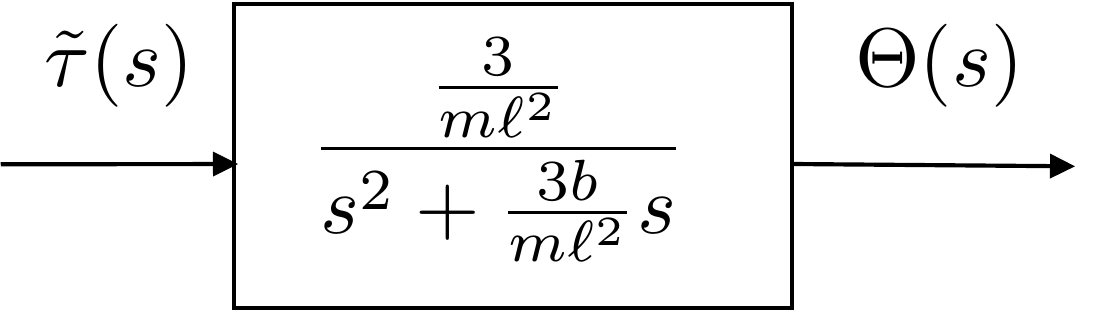
The block diagram associated with Equation 5.2 is shown in
Fig.5.1.
Figure 5.1. A block diagram of the single-link robot
arm.
5.3 SIMO Systems and Cascade
Approximations
There are many systems that have multiple inputs and/or multiple
outputs. In this case, a transfer function exists from each input
to each output. For example, suppose that the system is given by the
coupled differential equations \[\begin{aligned}
\ddot{y}_1 + a_{11}\dot{y}_1 + \ddot{y}_2 + a_{12}\dot{y}_2 &=
b_{11}u_1 + b_{12}u_2 + b_{13}\dot{u}_2 \\
\ddot{y}_2 + a_{22}y_2 &= b_{21}u_2.
\end{aligned}\] Taking the Laplace transform and arranging in
matrix notation gives \[\left(\begin{array}{c|c}
s^2+a_{11}s & s^2+a_{12}s \\ \hline 0 &
s^2+a_{22}\end{array}\right)
\begin{pmatrix}Y_1(s) \\ Y_2(s)\end{pmatrix} \\ =
\left(\begin{array}{c|c} b_{11} & (b_{13}s+b_{12}) \\ \hline0 &
b_{21}\end{array}\right)
\begin{pmatrix} U_1(s) \\ U_2(s)\end{pmatrix}.\] To find the
relevant transfer functions, we need to isolate the outputs on the
left-hand side by inverting the matrix on the left. Using the inverse
formula for a \(2\times 2\) matrix
derived in
Appendix 31\[\begin{pmatrix} a & b \\ c & d
\end{pmatrix}^{-1} = \frac{\begin{pmatrix} d & -b \\ -c &
a\end{pmatrix}}{ad-bc}\] we get \[\begin{aligned}
\begin{pmatrix}Y_1 \\ Y_2\end{pmatrix}
&= \left(\begin{array}{c|c} s^2+a_{11}s & s^2+a_{12}s \\ \hline
0 & s^2+a_{22}\end{array}\right)^{-1}
\left(\begin{array}{c|c} b_{11} & b_{13}s+b_{12} \\ \hline 0 &
b_{21}\end{array}\right)
\begin{pmatrix} U_1 \\ U_2\end{pmatrix} \\
&= \frac{\left(\begin{array}{c|c} s^2+a_{22} & -s^2-a_{12}s \\
\hline 0 & s^2+a_{11}s\end{array}\right)}{(s^2+a_{11}s)(s^2+a_{22})}
\left(\begin{array}{c|c} b_{11} & b_{13}s+b_{12} \\ \hline 0 &
b_{21}\end{array}\right)
\begin{pmatrix} U_1 \\ U_2\end{pmatrix} \\
&= \frac{\left(\begin{array}{c|c} b_{11}(s^2+a_{22}) &
(s^2+a_{22})(b_{13}s+b_{12})-b_{21}(s^2+a_{12}s) \\ \hline 0 &
b_{21}(s^2+a_{11}s)\end{array}\right)}{(s^2+a_{11}s)(s^2+a_{22})}
\begin{pmatrix} U_1 \\ U_2\end{pmatrix} \\
&= \left(\begin{array}{c|c} \frac{b_{11}}{s^2+a_{11}s} &
\frac{b_{13}s^3+(b_{12}-b_{21})s^2+(b_{13}a_{22}-b_{21}a_{12})s+a_{22}b_{12}}{(s^2+a_{11}s)(s^2+a_{22})}
\\ \hline 0 & \frac{b_{21}}{s^2+a_{22}}\end{array}\right)
\begin{pmatrix} U_1 \\ U_2\end{pmatrix}.
\end{aligned}\] Therefore, the transfer function from \(u_1\) to \(y_1\) is \(\frac{b_{11}}{s^2+a_{11}s}\), the transfer
function from \(u_2\) to \(y_1\) is \(\frac{b_{13}s^3+(b_{12}-b_{21})s^2+(b_{13}a_{22}-b_{21}a_{12})s+a_{22}b_{12}}{(s^2+a_{11}s)(s^2+a_{22})}\),
the transfer function from \(u_1\) to
\(y_2\) is \(0\), and the transfer function from \(u_2\) to \(y_2\) is \(\frac{b_{21}}{s^2+a_{22}}\).
For many of the case studies that we will look at in this book, there
is a single input, but we are also interested in controlling two or more
measurements or outputs. State-space control techniques are able to
create control laws to control multiple outputs in a single design step,
as we will see in later chapters. However, we also want to be able to
create single-input, multiple-output controllers using more classical
transfer-function based approaches. Doing so will require more intuition
about the systems we are controlling, as well as a clear understanding
of our control objectives so that we can make appropriate design
decisions and simplifying assumptions.
The majority of our design studies (specifically studies B, C, E, and
F) have coupled, higher-order dynamics (greater than order two) with
multiple outputs. Instead of coming up with a single feedback loop to
control the multiple outputs of interest, we will form a cascade of two
lower-order transfer functions and design two independent control loops.
Forming the cascade of lower-order transfer functions requires insights
into the dynamic behavior of the system, because it may require
simplifying assumptions about the dynamic coupling between the two
subsystems. Instead of a two-way coupling, the cascade may make the
dynamic coupling one-way. To reduce the complexity of the system, we may
make simplifying assumptions about the dynamics of one of the
subsystems. It is essential for these simplifications to be justifiable
given the parameters of the system and our control objectives. For
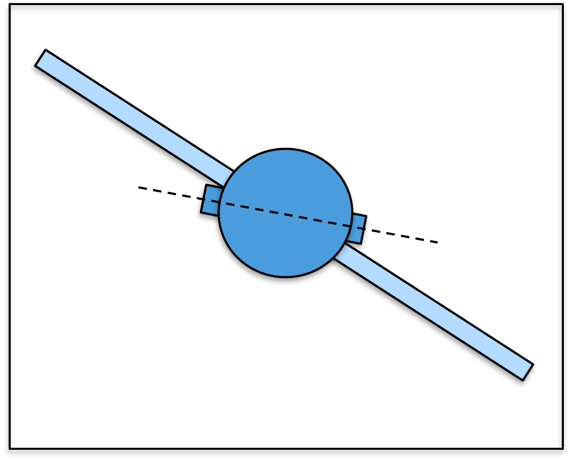
example, in design study C, we form a cascade of two transfer functions:
the first is from the torque input to the satellite angular position and
the second is from the satellite angular position to the solar panel
angular position. Because the satellite is more massive than the solar
panels, we will make a valid assumption that while the satellite
significantly influences the dynamic behavior of the solar panels, the
solar panels do not significantly influence the dynamic behavior of the
satellite. As we will see, this will simplify the design of the control
system significantly and result in a viable control design that provides
good performance.
In forming cascades of transfer functions, other factors may
influence the form of the cascade. Our control priorities may play a
significant role. For example, in design study B, the balancing of the
inverted pendulum is the highest priority and therefore, we will use the
force input to control the angle of the pendulum. Of importance, but
lower priority, is controlling the cart. These considerations will lead
us to form the cascade using the transfer functions from force to
pendulum angle and from pendulum angle to cart position. In other
situations, the causality of the dynamic behavior is more transparent.
In the block-beam system, the force on the beam causes the beam angle to
change and the change in beam angle causes the block to slide. We will
form the transfer function cascade for the block-beam system
accordingly. In the planar VTOL aircraft system, torque from the
differential thrust causes the aircraft to pitch, while thrust combined
with non-zero pitch causes the aircraft to translate. It is natural,
therefore, to think of torque causing pitch, and pitch causing
translational motion. We will thus form a cascade of two transfer
functions: from torque to pitch angle and from pitch angle to horizontal
position.
In forming a cascade of two (or more) transfer functions to represent
the dynamics of a single system, it is critically important that we
consider the physics of the system and our control objectives as we make
simplifying assumptions. Important questions to consider include:
What is the control input to the system?
What outputs of the system are to be controlled?
What outputs can be measured?
What physically justifiable simplifications can be made about the
dynamic coupling between subsystems?
What physically justifiable simplifying assumptions can be made
about the dynamics of the system?
Asking and answering these questions is fundamental to the design of
successful control systems. The more insight you have into the physical
behavior of the system you are controlling, the better your control
system designs will be.
(a) Start with the linearized equations and use the Laplace transform to
convert the equations of motion to the s-domain.
(b) Find the transfer functions from the input \(\tilde{F}(s)\) to the outputs \(\tilde{Z}(s)\) and \(\tilde{\Theta}(s)\). Assume that the
damping constant is negligible. How does this simplify the transfer
functions? Is this a reasonable assumption?
(c) From the simplified \(\tilde{Z}(s)/\tilde{F}(s)\) and \(\tilde{\Theta}(s)/\tilde{F}(s)\) transfer
functions, compute the \(\tilde{Z}(s)/\tilde{\Theta}(s)\) transfer
function. Draw a block diagram of the system as a series of two transfer
functions from \(\tilde{F}(s)\) to
\(\tilde{\Theta}(s)\) and from \(\tilde{\Theta}(s)\) to \(\tilde{Z}(s)\).
(d) Describe how this transfer-function cascade makes sense physically. How
does force influence the pendulum angle? How does the pendulum angle
influence the cart position?
Design
Study B guided exercise
Build the pendulum transfer-function
cascade
Start from the linearized equations and identify the
force-to-angle and angle-to-position relationship.
Use the cascade structure to separate the
fast force-to-angle subsystem from the angle-to-position
subsystem.
Step 1. Simplifying assumption
Show solution for Step
1
Answer: The transfer functions
are simplified by assuming b is negligible.
Step 2.
Force-to-angle subsystem
Show
solution for Step 2
Answer: The
upright pendulum force-to-angle dynamics include an unstable
right-half-plane pole.
Step
3. Angle-to-position subsystem
Show solution for Step
3
Answer: The angle-to-position
transfer function has two free integrators and produces cart position
z.
Complete solution
From HW 3.2.4, the linearized equations of
motion are given by \[\begin{pmatrix}
(m_1+m_2) & m_1 \frac{\ell}{2} \\
m_1 \frac{\ell}{2} & m_1 \frac{\ell^2}{3}
\end{pmatrix}\begin{pmatrix}
\ddot{\tilde{z}} \\ \ddot{\tilde{\theta}} \end{pmatrix} =
\begin{pmatrix} -b\dot{\tilde{z}} + \tilde{F}
\\
m_1 g \frac{\ell}{2} \tilde{\theta} \end{pmatrix}.\] The
second equation in this matrix formulation can be simplified by dividing
both sides of the second equation by \(m_1
\frac{\ell}{2}\) to give \[\begin{pmatrix} (m_1+m_2) & m_1
\frac{\ell}{2} \\
1 & \frac{2 \ell}{3} \end{pmatrix}\begin{pmatrix}
\ddot{\tilde{z}} \\ \ddot{\tilde{\theta}} \end{pmatrix} =
\begin{pmatrix} -b\dot{\tilde{z}} + \tilde{F}
\\
g \tilde{\theta} \end{pmatrix}.\] We can write these
equations with states and state derivatives on the left and inputs on
the right as \[\begin{aligned}
(m_1+ m_2) \ddot{\tilde{z}} + m_1\frac{\ell}{2} \ddot{\tilde{\theta}} +
b\dot{\tilde{z}} &= \tilde{F} \\
\ddot{\tilde{z}} + \frac{2\ell}{3} \ddot{\tilde{\theta}} -
g{\tilde{\theta}} &= 0 .
\end{aligned}\] Taking the Laplace transform gives \[\begin{aligned}
\left[ (m_1+m_2) s^2 + b s \right] \tilde{Z}(s) + m_1\frac{\ell}{2} s^2
\tilde{\Theta}(s) &= \tilde{F}(s) \\
s^2 \tilde{Z}(s) + \left(\frac{2 \ell}{3} s^2 - g
\right)\tilde{\Theta}(s) &= 0 .
\end{aligned}\] These equations can be expressed in matrix form
as \[\begin{pmatrix} (m_1+m_2)s^2 + bs &
m_1 \frac{\ell}{2}s^2 \\
s^2 & \frac{2 \ell}{3}s^2-g \end{pmatrix}\begin{pmatrix}
\tilde{Z}(s) \\ \tilde{\Theta}(s) \end{pmatrix} =
\begin{pmatrix} \tilde{F}(s) \\
0 \end{pmatrix}.\] Inverting the matrix on the left-hand side
and solving for the transfer functions gives \[\begin{aligned}
\tilde{Z}(s) &= \left(\frac{ \frac{2 \ell}{3} s^2 - g}{(m_1
\frac{\ell}{6}+ m_2 \frac{2 \ell}{3}) s^4 +b\frac{2\ell}{3} s^3
-(m_1+m_2)gs^2-bgs}\right) \tilde{F}(s) \\
\tilde{\Theta}(s) &= \left(\frac{-s^2}{(m_1 \frac{\ell}{6}+ m_2
\frac{2 \ell}{3}) s^4 +b\frac{2\ell}{3} s^3 -(m_1+m_2)gs^2-bgs}\right)
\tilde{F}(s).
\end{aligned}\]
If we make the assumption that \(b \approx
0\), then these transfer functions will simplify further and be
even easier to work with from a control design perspective. This is a
reasonable and conservative assumption because the damping force \(b\dot{z}\) is small relative to the other
forces acting on the system. Furthermore, by underestimating the damping
in the system, our control design will be conservative because it
assumes there is no damping provided by the physics of the system and
thus all the damping in the system must come from the feedback control.
Assuming \(b=0\), we get \[\begin{aligned}
\tilde{Z}(s) &= \left(\frac{\frac{2 \ell}{3} s^2 - g}{s^2\left[(m_1
\frac{\ell}{6}+ m_2 \frac{2 \ell}{3}) s^2 -(m_1+m_2)g \right]}\right)
\tilde{F}(s) \\
\tilde{\Theta}(s) &= \left(\frac{-1}{(m_1 \frac{\ell}{6}+ m_2
\frac{2 \ell}{3}) s^2 -(m_1+m_2)g}\right) \tilde{F}(s).
\end{aligned}\]
From a control-systems perspective, we will be interested in how the
pendulum angle \(\theta\) influences
the cart position \(z\), and so we want
to find the transfer function from \(\tilde{\Theta}(s)\) to \(\tilde{Z}(s)\). This can be easily
calculated by recognizing that \[\tilde{Z}(s)
=
\frac{\tilde{Z}(s)}{\tilde{F}(s)}\frac{\tilde{F}(s)}{\tilde{\Theta}(s)}
\tilde{\Theta}(s).\] Accordingly, \[\tilde{Z}(s) = \left(\frac{-\frac{2 \ell}{3} s^2
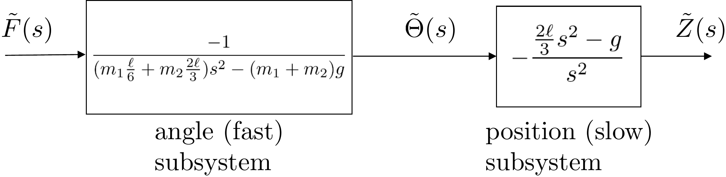
+ g}{s^2} \right) \tilde{\Theta}(s).\] The block diagram for the
approximate system is shown in Figure 5.2.
Figure 5.2. The inverted pendulum dynamics are
approximated by a cascade of fast and slow subsystems. The fast
subsystem is the transfer function from the force to the angle, and the
slow subsystem is the transfer function from the angle to the
position.
This transfer function cascade makes sense physically. With the
pendulum balanced vertically, a positive force on the cart would cause
the pendulum to fall in the negative direction as indicated by the minus
sign in the numerator. The pendulum falls in an unstable motion due to
the right-half-plane pole in the transfer function. The angle of the rod
influences the position of the cart as shown in the second transfer
function. If the pendulum were balanced vertically with no input force
applied and a small disturbance caused the pendulum to fall in the
positive direction, the cart would shoot off in the negative direction.
Again, this can be seen from the negative sign in the numerator of the
transfer function and the right-half-plane pole in the denominator. Keep
in mind that these equations are linearized about the vertical position
of the pendulum. When the pendulum is hanging down, the equations are
different. How are they different?
The PID and loopshaping techniques that we will discuss in
Parts III
and V will use the
approximate transfer function models of the plant derived above. The
state-space methods discussed in
Part IV will use
a state-space model, which does not depend on neglecting the coupling
between subsystems and does not depend on a separation into fast and
slow subsystems.
(a) Start with the linearized equations for the satellite attitude problem
and use the Laplace transform to convert the equations of motion to the
s-domain.
(b) Find the full transfer matrix from the input \(\tau(s)\) to the outputs \(\Phi(s)\) and \(\Theta(s)\).
(c) From the transfer matrix, find the second-order transfer function from
\(\Theta(s)\) to \(\Phi(s)\).
(d) Under the assumption that the panel moment of inertia \(J_p\) is significantly smaller than the
spacecraft moment of inertia \(J_s\)
(specifically, \((J_s+J_p)/J_s \approx
1\)), find the second-order approximation for the transfer
function from \(\tau(s)\) to \(\Theta(s)\).
(e) From your results on parts (c) and (d), form the approximate transfer
function cascade for the satellite/panel system and justify why it makes
sense physically.
Design Study C guided exercise
Build the satellite transfer-function cascade
The
transfer-function model separates the body-angle dynamics from the
panel-angle dynamics using a physically motivated cascade
approximation.
The approximation lets the body angle drive
the panel dynamics while neglecting the panel's back-effect on the
massive satellite body.
Step 1. Identify the s-domain outputs
Show solution for Step
1
Answer: The transfer matrix maps
\(\tau(s)\) to \(\Theta(s)\) and \(\Phi(s)\).
Step 2.
Body angle to panel angle
Show
solution for Step 2
Answer: The
panel subsystem is \(P_{out}(s)=\Phi(s)/\Theta(s)\), a second-order
flexible-mode transfer function.
Step 3.
Torque to body angle approximation
Show solution for Step
3
Answer:\(P_{in}(s)=\Theta(s)/\tau(s)\approx 1/((J_s+J_p)s^2)\),
so the approximate body plant has two free
integrators.
Step 4. Interpret the approximation
Show solution for Step
4
Answer: The cascade assumes the
satellite body significantly influences the panel, while the panel does
not significantly influence the satellite body.
Complete solution
From HW 3.3.3, the linearized equations of
motion are given by \[\begin{pmatrix}\ddot{\theta} \\ \ddot{\phi}
\end{pmatrix}
= \begin{pmatrix}
-\frac{b}{J_s}(\dot{\theta}-\dot{\phi})-\frac{k}{J_s}(\theta-\phi)+\frac{1}{J_s}\tau
\\ -\frac{b}{J_p}(\dot{\phi}-\dot{\theta}) -\frac{k}{J_p}(\phi-\theta)
\end{pmatrix}\] or in other words, the coupled differential
equations \[\begin{aligned}
\ddot{\theta} + \frac{b}{J_s}\dot{\theta} + \frac{k}{J_s}\theta &=
\frac{b}{J_s}\dot{\phi}+\frac{k}{J_s}\phi+\frac{1}{J_s}\tau \\
\ddot{\phi} + \frac{b}{J_p}\dot{\phi} +\frac{k}{J_p}\phi &=
\frac{b}{J_p}\dot{\theta} + \frac{k}{J_p}\theta.
\end{aligned}\] Taking the Laplace transform with initial
conditions set to zero and rearranging gives \begin{align}
(s^2+\frac{b}{J_s}s+\frac{k}{J_s})\Theta(s) &=
(\frac{b}{J_s}s+\frac{k}{J_s})\Phi(s)+\frac{1}{J_s}\tau(s)
\tag{5.3}\\
(s^2+\frac{b}{J_p}s+\frac{k}{J_p})\Phi(s) &=
(\frac{b}{J_p}s+\frac{k}{J_p})\Theta(s).
\tag{5.4}
\end{align}
To find the transfer matrix from \(\tau\) to \((\Theta, \Phi)^\top\), write Equation 5.3 and 5.4 in matrix form as \[\left(\begin{array}{c|c}
s^2+\frac{b}{J_s}s+\frac{k}{J_s} & -\frac{b}{J_s}s-\frac{k}{J_s}
\\\hline
-\frac{b}{J_p}s-\frac{k}{J_p} & s^2+\frac{b}{J_p}s+\frac{k}{J_p}
\end{array}\right)
\begin{pmatrix}\Theta(s) \\ \Phi(s) \end{pmatrix}
= \begin{pmatrix} \frac{1}{J_s} \\ 0 \end{pmatrix} \tau(s),\] and
invert the matrix on the left-hand side to obtain \[\begin{pmatrix}\Theta(s) \\ \Phi(s) \end{pmatrix}
= \begin{pmatrix}
\frac{\frac{1}{J_s}s^2+\frac{b}{J_sJ_p}s+\frac{k}{J_sJ_p}}{s^2\left(
s^2+\frac{b(J_s+J_p)}{J_sJ_p}s+\frac{k(J_s+J_p)}{J_sJ_p} \right)}
\\
\frac{\frac{b}{J_sJ_p}s+\frac{k}{J_sJ_p}}{s^2\left(
s^2+\frac{b(J_s+J_p)}{J_sJ_p}s+\frac{k(J_s+J_p)}{J_sJ_p} \right)}
\end{pmatrix} \tau(s).\]
By dividing the bottom transfer function of the transfer matrix \(\Phi(s)/\tau(s)\) by the top transfer
function of the transfer matrix \(\Theta(s)/\tau(s)\), we can find the
transfer function from the satellite angular position to the panel
angular position \[\frac{\Phi(s)}{\Theta(s)}
= \frac{\frac{b}{J_p}s+\frac{k}{J_p}}{s^2+\frac{b}{J_p}s+\frac{k}{J_p}}.
\tag{5.5}\]
From the transfer matrix, the transfer function from \(\tau(s)\) to \(\Theta(s)\) is given by \[\frac{\Theta(s)}{\tau(s)} =
\frac{\frac{1}{J_s}s^2+\frac{b}{J_sJ_p}s+\frac{k}{J_sJ_p}}{s^2\left(
s^2+\frac{b(J_s+J_p)}{J_sJ_p}s+\frac{k(J_s+J_p)}{J_sJ_p}
\right)}\] Under the assumption that the moment of inertia of the
panel is significantly smaller than the inertia of the satellite (which
is true for this problem), we can infer that \((J_s+J_p)/J_s \approx 1\). Taking this into
account, we can simplify \(\Theta(s)/\tau(s)\) as \[\begin{aligned}
\frac{\Theta(s)}{\tau(s)} &=
\frac{\frac{1}{J_s}\left(s^2+\frac{b}{J_p}s+\frac{k}{J_p}\right)}{s^2
\left( \frac{J_s+J_p}{J_s} \right)\left( \frac{J_s}{J_s+J_p}
s^2+\frac{b}{J_p}s+\frac{k}{J_p} \right)} \\
&\approx \frac{1}{(J_s+J_p)s^2} .
\end{aligned}\]
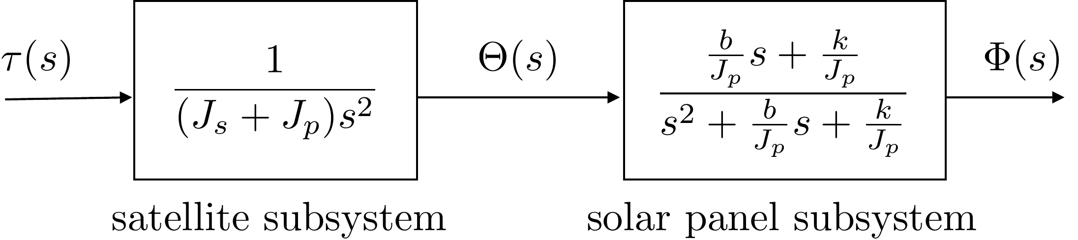
The block diagram for the approximate system is shown in Figure 5.3.
Figure 5.3. The satellite attitude dynamics are
approximated by a cascade of the satellite and panel
subsystems.
The cascade approximation has the exact transfer function for the
panel subsystem, but it has an approximate transfer function for the
satellite subsystem. The approximation implies that the dynamics of the
satellite affects the dynamics of the panel, but the dynamics of the
panel do not affect the dynamics of the satellite. Notice that the
transfer function for the satellite has the dynamics of a rigid body
with a moment of inertia of \(J_s+J_p\). As long as the moment of inertia
of the satellite is significantly greater than the moment of inertia of
the panel, this assumption is reasonable and approximates the fully
coupled dynamics of the system with acceptable accuracy.
5.6 Interactive Transfer Function
Check
Chapter 5 activity
Read a second-order transfer function
Adjust the coefficients in
H(s)=b0/(s2+a1s+a0) and
watch how the denominator determines poles while
b0/a0 sets the DC gain when a0 is
nonzero.
Transfer function
Poles
DC gain
System order
Transfer functions describe zero-initial-condition input-output
behavior. Poles come from the denominator roots; zeros come from
numerator roots.
5.7 Knowledge Check
Q1. Initial conditions
What initial-condition assumption is used when
forming a transfer function?
Q2.
Poles
Where do the poles of a transfer
function come from?
Q3. DC gain
For H(s)=6/(s2+4s+3), enter the DC gain H(0).
Show solution
Answer: 2, because H(0)=6/3.
Q4. First-order pole
For the denominator s+4, enter the pole location.
Show solution
Answer: -4, because s+4=0 gives s=-4.
Q5. Numerator roots
What are the roots of a transfer function numerator called?
Show solution
Answer: They are zeros.
Q6. Transfer-function assumption
Which assumption is used when deriving a transfer
function from a differential equation?
Q7. Pole-zero identification
For G(s)=(s+4)/((s+1)(s+3)), which statement is
correct?
Q8. DC
gain
For stable
G(s)=(s+2)/(s2+6s+8), what final value should a unit step
input approach?
Q9. Cascade approximation
When is a cascade approximation most
useful?
5.8 Notes and References
The Laplace transform can be found in introductory textbooks on
signals and systems like [16] and in introductory textbooks on
differential equations. The transfer function of a linear time-invariant
system is also covered in introductory textbooks on signals and systems,
and in most introductory textbooks on control like [4].