P.3 Simulating Control Systems Using Simulink

In this appendix we will show how to simulate the feedback control of a dynamic system using Simulink. Consider the general feedback control system shown in Figure 3.1. The output of the physical system is \(y(t)\), and the inputs to the physical system are \(u(t)\) and an external disturbance signal \(d(t)\). The output of the system \(y(t)\) is corrupted by zero-mean noise \(n(t)\). The inputs to the controller are the reference signal \(r(t)\) and the output corrupted by noise.

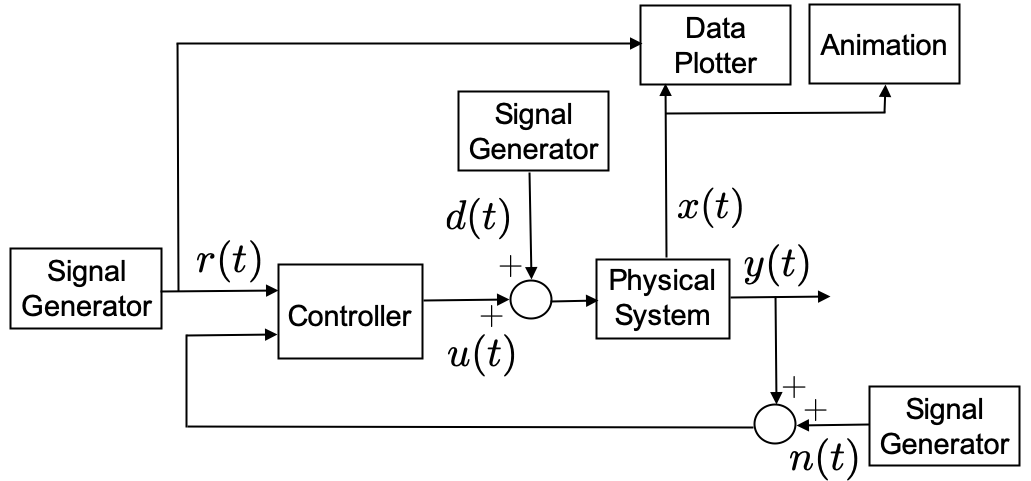
We will illustrate how to implement feedback control systems in Simulink by simulating the physical system described by the differential equation \[\tag{P.3.1} \ddot{y} + 2\dot{y} + 3 y = 4 u,\] and using the PID controller \[\tag{P.3.2} u(t) = k_p (r(t)-y(t)) + k_i \int_{-\infty}^t (r(\tau)-y(\tau))d\tau - k_d \dot{y}.\]

The Simulink diagram that corresponds to Figure 3.1 is shown in Figure 3.2.

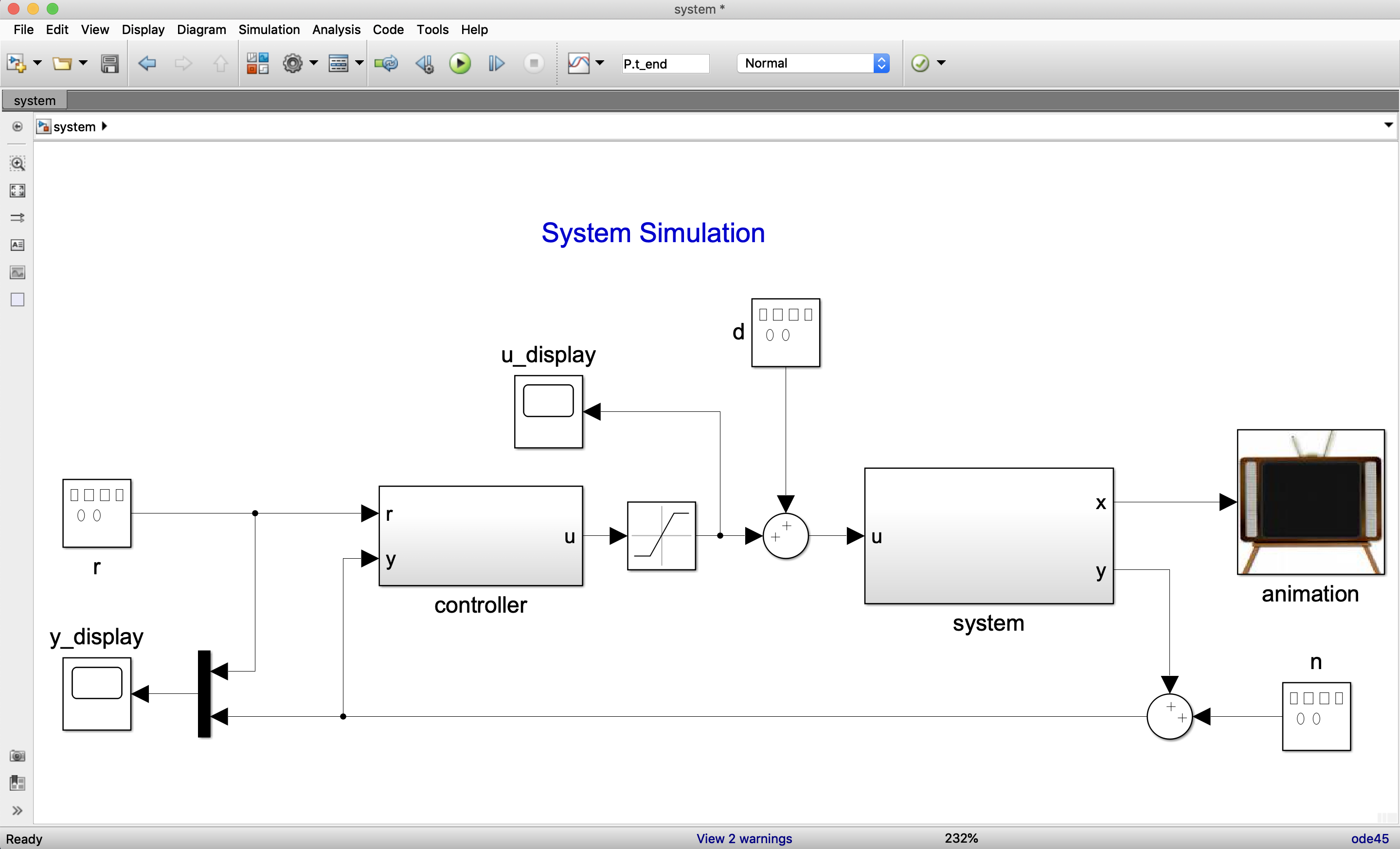
The system dynamics are implemented in the system block, the controller is implemented in the controller block, and the animation is implemented in the animation block. The reference \(r(t)\), the disturbance \(d(t)\), and the noise \(n(t)\) are all implemented using the built-in Simulink Signal Generator block. The built-in Simulink Scope blocks are used to display the output \(y\) and the reference \(r\), as well as the input \(u\).

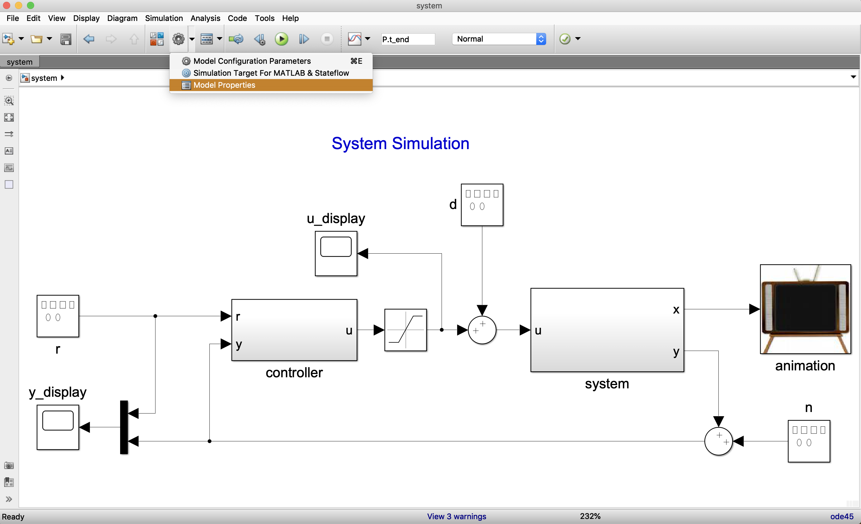
System parameters can be loaded into Simulink at the beginning of a simulation by clicking on the Model Properties menu, as shown in Figure 3.3,

and then selecting Callbacks/InitFcn, as shown in Figure 3.4.

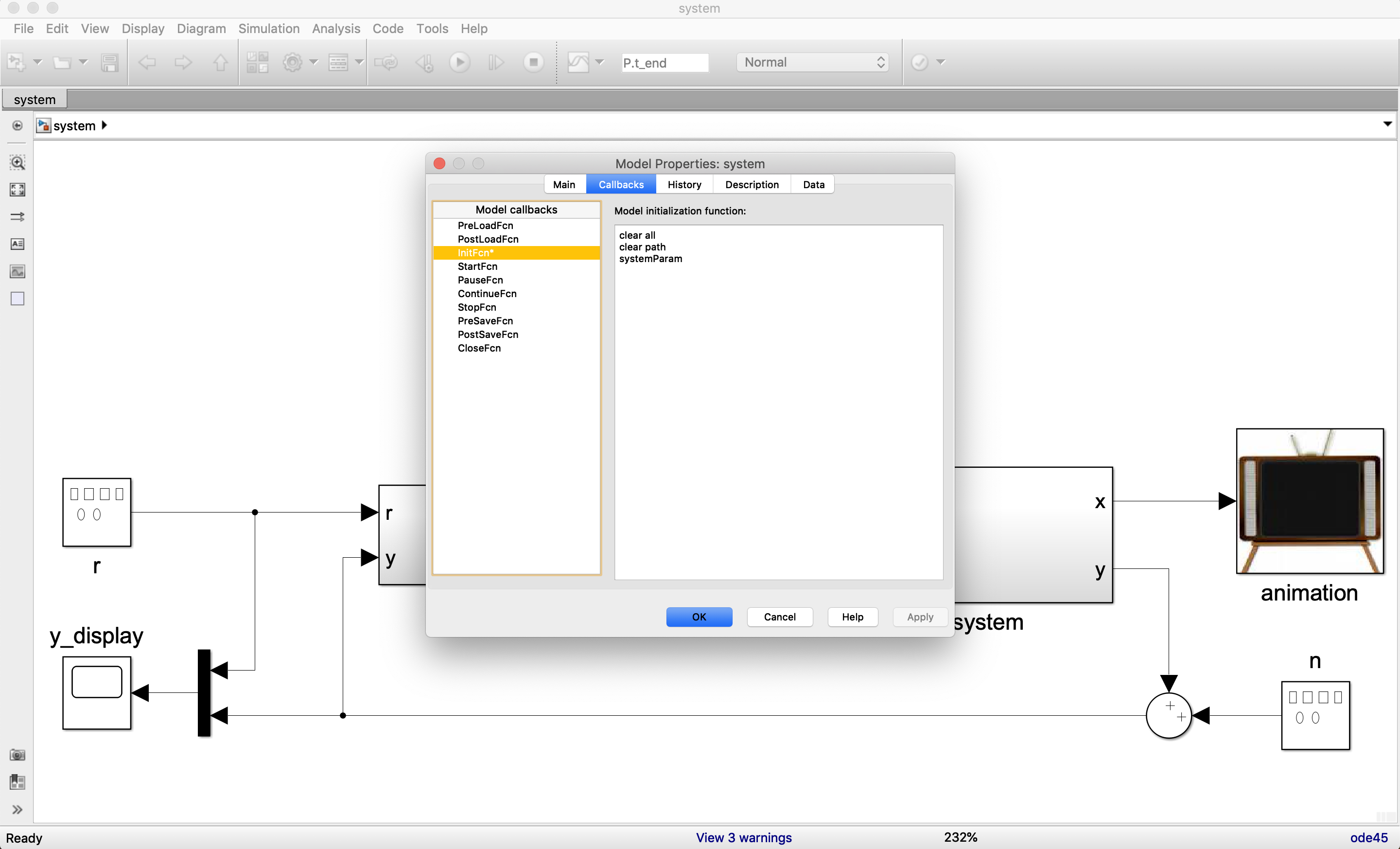
The commands listed under Model initialization function: are executed at the beginning of each Simulink simulation.

P.3.1 System Dynamics

In this section we will describe how to implement the system dynamics. Double-clicking the system block shown in Figure 3.2 results in the Simulink sub-diagram shown in Figure 3.5.

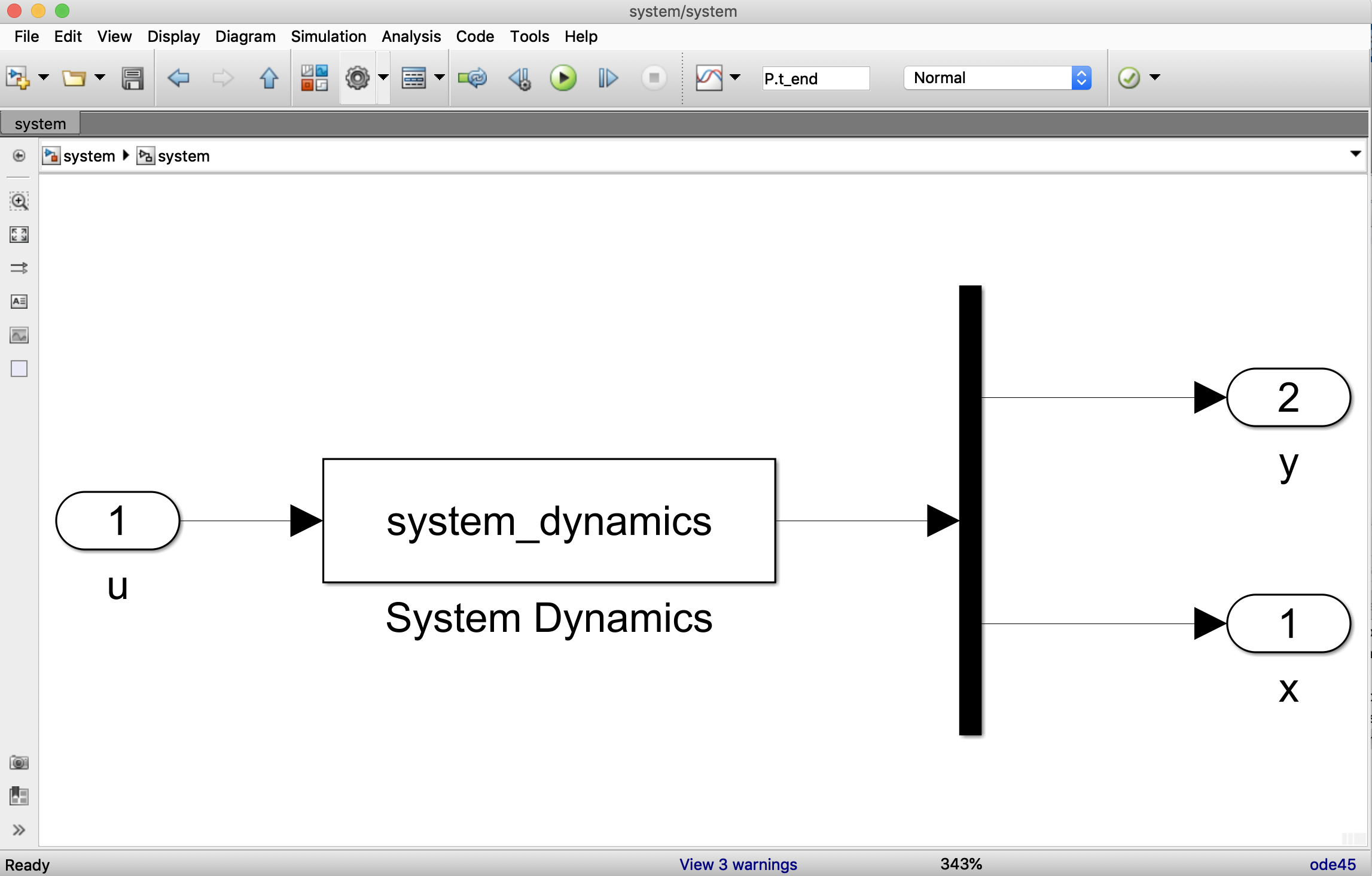
Double-clicking the System Dynamics block results in Figure 3.6, which shows an s-function dialog block.

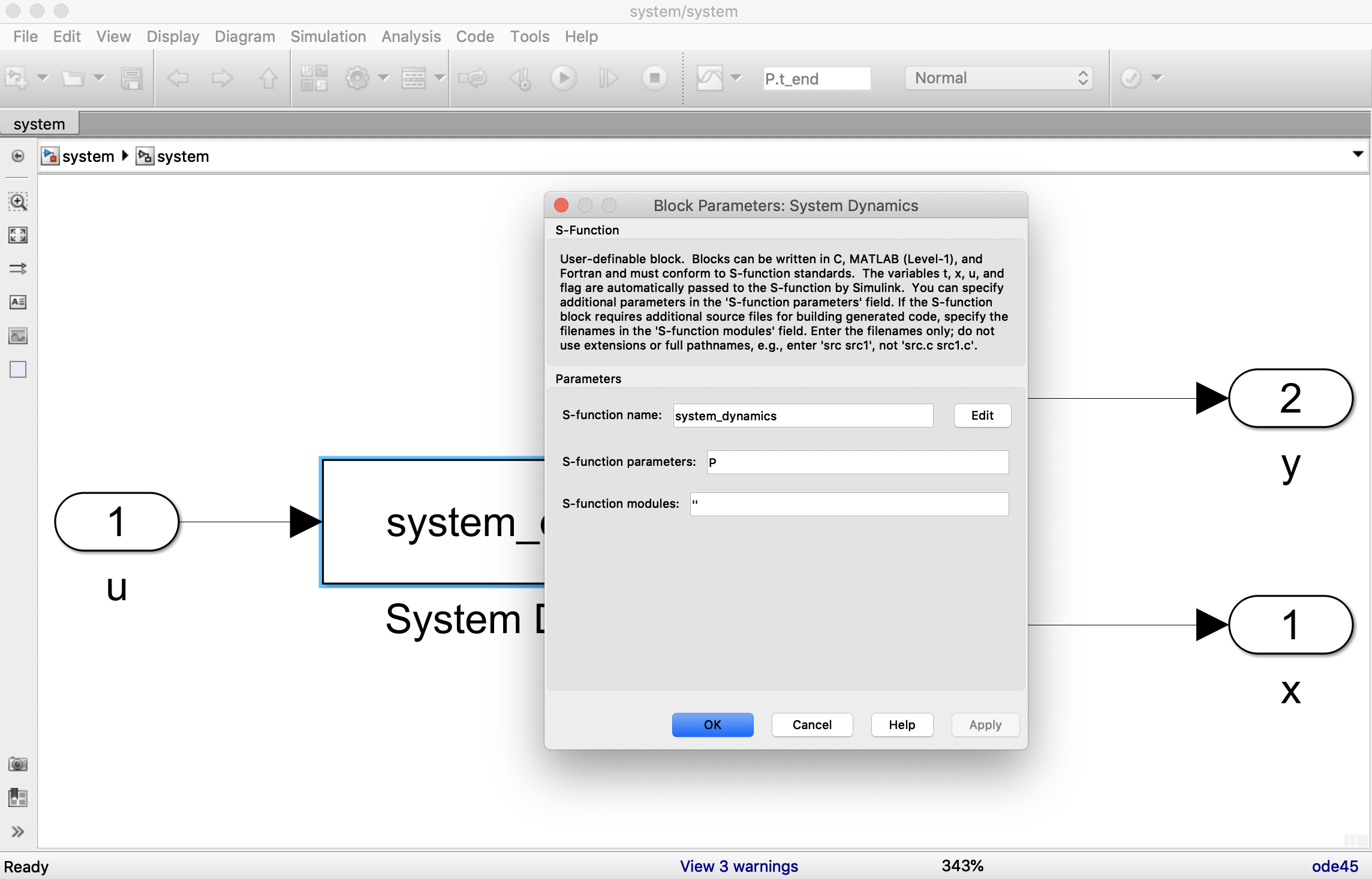
In Simulink, system dynamics are implemented using s-functions. Simulink is essentially a sophisticated tool for solving interconnected hybrid ordinary differential and difference equations. Each block in Simulink is assumed to have the structure \begin{align} \dot{x}_c &= f(t, x_c, x_d, u); \qquad x_c(0) = x_{c0} \tag{P.3.3} \\ x_d[k+1] &= g(t, x_c, x_d, u); \qquad x_d[0] = x_{d0} \tag{P.3.4} \\ y &= h(t, x_c, x_d, u) \tag{P.3.5} , \end{align} where \(x_c\in{\mathbb{R}}^{n_c}\) is a continuous state with initial condition \(x_{c0}\), \(x_d\in{\mathbb{R}}^{n_d}\) is a discrete state with initial condition \(x_{d0}\), \(u\in{\mathbb{R}}^m\) is the input to the block, \(y\in{\mathbb{R}}^p\) is the output of the block, and \(t\) is the elapsed simulation time. An s-function is a Simulink tool for explicitly defining the functions \(f\), \(g\), and \(h\) and the initial conditions \(x_{c0}\) and \(x_{d0}\). As explained in the MATLAB/Simulink documentation, there are several methods for specifying an s-function. In this section, we provide an overview of the method that uses a Level-1 M-file s-function.

The system given in Equation P.3.1 is implemented using the s-function shown below.

function [sys,x0,str,ts,simStateCompliance]...
    =system_dynamics(t,x,u,flag)
switch flag
  case 0  % Initialize block
    [sys,x0,str,ts,simStateCompliance]=mdlInitializeSizes;
  case 1  % define xdot = f(t,x,u)
    sys=mdlDerivatives(t,x,u);
  case 3  % define y = h(t,x,u)
    sys=mdlOutputs(t,x,u);
  % GetTimeOfNextVarHit 
  otherwise
    DAStudio.error(...
        'Simulink:blocks:unhandledFlag',num2str(flag));
end
%==============================================
function [sys,x0,str,ts,simStateCompliance]=mdlInitializeSizes
sizes = simsizes;
sizes.NumContStates  = 2;
sizes.NumDiscStates  = 0;
sizes.NumOutputs     = 1+2;
sizes.NumInputs      = 1;
sizes.DirFeedthrough = 0;
sizes.NumSampleTimes = 1;   
sys = simsizes(sizes);

% define initial conditions
y0 = 0;  % initial condition for y
ydot0 = 0;  % initial condition for ydot
x0  = [y0; ydot0];
str = [];  % str is always an empty matrix
% initialize the array of sample times
ts  = [0 0];
simStateCompliance = 'UnknownSimState';

%==============================================
function sys=mdlDerivatives(t,x,u)
    % Return xdot = f(x,u)
    y = x(1);
    ydot = x(2);

    % system parameters
    persistent a0
    persistent a1
    persistent b0
    if t==0
        a0 = 3.0;
        a1 = 2.0;
        b0 = 4.0;
        % modify the system parameters by random value
        alpha = 0.2;  % Uncertainty parameter
        a0 = a0 * (1+2*alpha*rand-alpha);  
        a1 = a1 * (1+2*alpha*rand-alpha);  
        b0 = b0 * (1+2*alpha*rand-alpha); 
    end
    % The equations of motion.
    yddot = -a1 * ydot - a0 * y + b0 * u;
    % build xdot and return
    sys = [ydot; yddot];

%==============================================
function sys=mdlOutputs(t, x, u)
    y = x(1);
    sys = [y; x];  % return output and state

Lines 1–2 define the main s-function file. The inputs to this function are always the elapsed time \(t\); the state \(x\), which is a concatenation of the continuous state and discrete state; the input \(u\); and a flag, followed by user-defined input parameters, which are absent in this case. The Simulink engine calls the s-function and passes the parameters \(t\), \(x\), \(u\), and flag. When flag==0, the Simulink engine expects the s-function to return the structure sys, which defines the block; initial conditions x0; an empty string str; and an array ts that defines the sample times of the block. When flag==1, the Simulink engine expects the s-function to return the function \(f(t,x,u)\), and when flag==3, the Simulink engine expects the s-function to return \(h(t,x,u)\). The switch statement that calls the proper functions based on the value of flag is shown in Lines 3–13. The block setup and the definition of the initial conditions are shown in Lines 16–33. The numbers of continuous states, discrete states, outputs, and inputs are defined on Lines 18–21. The direct feedthrough term on Line 22 is set to one if the output depends explicitly on the input \(u\). For example, this occurs if \(D\neq 0\) in the linear state-space output equation \(y=Cx+Du\). The initial conditions are defined on Lines 26–29. The sample times are defined on Line 32. The format for this line is ts = [period offset], where period defines the sample period and is \(0\) for continuous time or \(-1\) for inherited, and where offset is the sample time offset, which is typically \(0\). The function \(f(t,x,u)\) is defined in Lines 36–58, and the output function \(h(t,x,u)\) is defined in Lines 61–63.

P.3.2 Controller

In this section we will describe how to implement the controller. Double-clicking the controller block shown in Figure 3.2 results in the Simulink sub-diagram shown in Figure 3.7, which also shows the pop-up window that results from clicking the Interpreted MATLAB Function block.

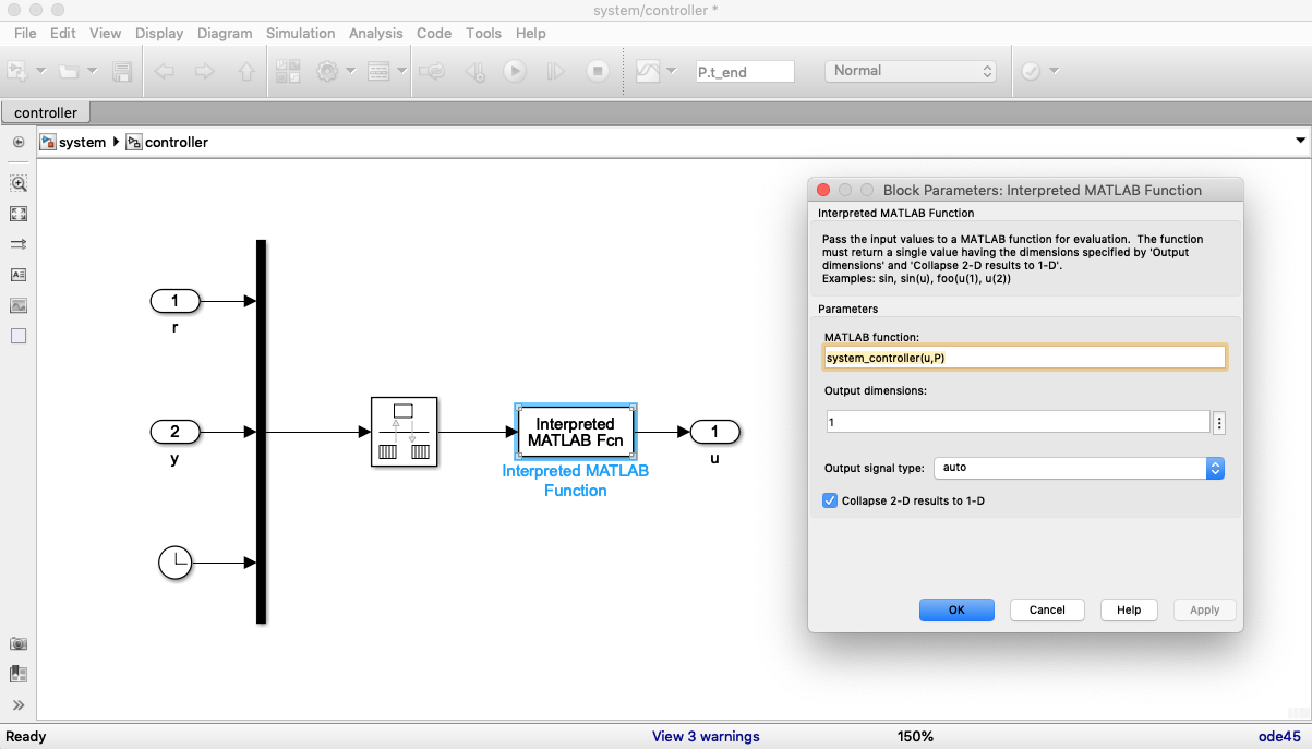
This block calls the MATLAB function system_controller.m with inputs u, coming into the Simulink block, and the parameter structure P, which must be defined in the MATLAB workspace. The m-file that defines the controller is listed below.

function u=system_controller(in, Ts)
    r   = in(1);
    y   = in(2);
    t   = in(3);
    % controller gains
    kp = 1;
    kd = 1;
    ki = 1;
    sigma = 2*Ts;
    beta = (2*sigma-Ts)/(2*sigma+Ts);
    limit = 1;
    
    % define the error
    error = r - y;  
    
    % set persistent variables at start of simulation
    persistent integrator
    persistent ydot
    persistent error_d1
    persistent y_d1
    if t<Ts
        integrator = 0;
        ydot = 0;
        error_d1 = error;
        y_d1 = y;
    end
    
    % update the integrator
    integrator = integrator + (Ts/2)*(error+error_d1);
    % update the derivative of y
    ydot = beta*ydot + (1-beta)*(y-y_d1)/Ts;
    % form PID controller, saturate, and return
    u_unsat = kp*error + ki*integrator - kd*ydot;
    u = saturate(u_unsat, limit);
    % update persistent delay variables
    error_d1 = error;
    y_d1 = y;
end
    
%-----------------------------------------------------------------
% saturation function
function out = sat(in,limit)
    if     in > limit,      out = limit;
    elseif in < -limit,     out = -limit;
    else                    out = in;
    end
end

The inputs to system_controller.m are in and the sample rate Ts. The input array is decomposed into the reference \(r\), the system output \(y\), and the time \(t\) on lines 2–4. The controller gains are set on lines 5–11, and the error is calculated on line 14. The persistent variables that must persist between function calls are defined and initialized on lines 16–26. The integrator is updated on line 29, the differentiator is updated on line 31, and the PID controller is specified on lines 33–34. The delay variables are updated on lines 36–37.

P.3.3 Animation

In this section we will show how to create an animation for the inverted pendulum case study in Simulink.

When a graphics function like plot is called in MATLAB, the function returns a handle to the plot. A graphics handle is similar to a pointer in C/C++ in the sense that all of the properties of the plot can be accessed through the handle. For example, the MATLAB command

    >> plot_handle=plot(t,sin(t))

returns a pointer, or handle, to the plot of sin(t). Properties of the plot can be changed by using the handle, rather than reissuing the plot command. For example, the MATLAB command

    >> set(plot_handle, 'YData', cos(t))

changes the plot to cos(t) without redrawing the axes, title, label, or other objects that may be associated with the plot. If the plot contains drawings of several objects, a handle can be associated with each object. For example,

    >> plot_handle1 = plot(t,sin(t))
    >> hold on
    >> plot_handle2 = plot(t,cos(t))

draws both sin(t) and cos(t) on the same plot, with a handle associated with each object. The objects can be manipulated separately without redrawing the other object. For example, to change cos(t) to cos(2t), issue the command

    >> set(plot_handle2, 'YData', cos(2*t))

We can exploit this property to animate simulations in Simulink by redrawing only the parts of the animation that change in time, and thereby significantly reducing the simulation time. To show how handle graphics can be used to produce animations in Simulink, we will show how to draw the inverted pendulum in a 2-D animation.

Consider the image of the inverted pendulum shown in Fig. 3.8, where the configuration is completely specified by the position of the cart \(z\), and the angle of the rod from vertical \(\theta\). The physical parameters of the system are the rod length \(\ell\), the base width \(w\), the base height \(h\), and the gap between the base and the track \(g\).

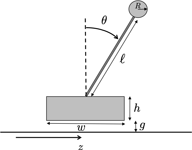
The first step in developing the animation is to determine the position of points that define the animation. For example, for the inverted pendulum in Fig. 3.8, the four corners of the base are \[(z+w/2, g), (z+w/2, g+h), (z-w/2, g+h), \text{ and } (z-w/2, g),\] and the two ends of the rod are given by \[(z, g+h) \text{ and } (z+L\sin\theta, g+h+L\cos\theta).\]

Since the base and the rod can move independently, each will need its own figure handle. The drawBase command can be implemented with the following MATLAB code:

function handle...
         = drawBase(z, width, height, gap, handle)
  X = [z-width/2,z+width/2,z+width/2,z-width/2];
  Y = [gap, gap, gap+height, gap+height];
  if isempty(handle),
    handle = fill(X,Y,'m');
  else
    set(handle,'XData',X,'YData',Y);
  end

Lines 2 and 3 define the X and Y locations of the corners of the base. Note that in Line 1, handle is both an input and an output. If an empty array is passed into the function, then the fill command is used to plot the base in Line 5. On the other hand, if a valid handle is passed into the function, then the base is redrawn using the set command in Line 7.

The MATLAB code for drawing the rod is similar and is listed below.

function handle...
         = drawRod(z,theta,L,gap,height,handle)
  X = [z, z+L*sin(theta)];
  Y = [gap+height, gap + height + L*cos(theta)];
  if isempty(handle),
    handle = plot(X, Y, 'g');
  else
    set(handle,'XData',X,'YData',Y);
  end

The main routine for the pendulum animation is listed below.

function drawPendulum(u)
  %
  z        = u(1);
  theta    = u(2);
  t        = u(3);

  %
  L = 1;
  gap = 0.01;
  width = 1.0;
  height = 0.1;

  %
  persistent base_handle
  persistent rod_handle

  %
  %
  if t==0,
    figure(1), clf
    track_width=3;
    %
    plot([-track_width,track_width],[0,0],'k'); 
    hold on
    base_handle...
       =drawBase(z, width, height, gap, []);
    rod_handle...
       =drawRod(z, theta, L, gap, height, []);
    axis([-track_width,track_width,...
          -L,2*track_width-L]);
  %
  else
    drawBase(z, width, height, gap, base_handle);
    drawRod(z, theta, L, gap, height, rod_handle);
  end

The routine drawPendulum is called from the Simulink file shown above, where there are three inputs: the position \(z\), the angle \(\theta\), and the time \(t\). Lines 3–5 rename the inputs to \(z\), \(\theta\), and \(t\). Lines 8–11 define the drawing parameters. We require that the handle graphics persist between function calls to drawPendulum. Since a handle is needed for both the base and the rod, we define two persistent variables in Lines 14 and 15. The if statement in Lines 19–32 is used to produce the animation. Lines 20–27 are called once at the beginning of the simulation, and draw the initial animation. Line 20 brings the figure 1 window to the front and clears it. Lines 21 and 23 draw the ground along which the pendulum will move. Line 25 calls the drawBase routine with an empty handle as input, and returns the handle base_handle to the base. Line 26 calls the drawRod routine, and Line 25 sets the axes of the figure. After the initial time step, all that needs to be changed are the locations of the base and rod. Therefore, in Lines 30 and 31, the drawBase and drawRod routines are called with the figure handles as inputs.