14 Disturbance Observers

14.1 Theory

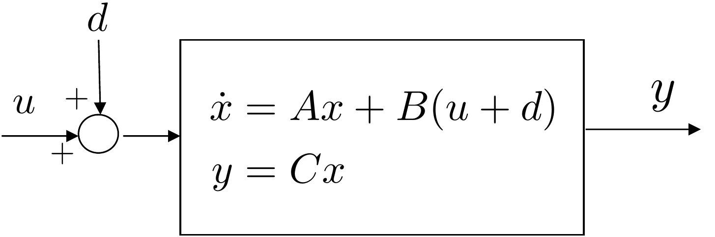
In previous sections we have discussed that modeling errors and other real-world effects result in an input disturbance to the system as shown in Fig. 14.1.

Figure 14.1. Input disturbance to plant modeled by state-space equations.

The objective of this section is to explain the effect of the disturbance on an observer. It turns out that the disturbance creates a steady-state bias in the observer states. We will also describe how the observer can be augmented to estimate the disturbance and to remove the steady-state observation error. This is the dual of adding an integrator to a state-space system.

To understand the effect of the disturbance on the observer, note that when the disturbance is present, the state-space equations for the system are \[\begin{aligned} \dot{x} &= Ax + B(u+d) \\ y &= C x. \end{aligned}\] The standard equation for the observer is \[\tag{14.1} \dot{\hat{x}} = A\hat{x} + Bu + L(y-C\hat{x}).\] Defining the observation error as \(e=x-\hat{x}\) and taking the derivative with respect to time gives \begin{align} \dot{e} &= \dot{x}-\dot{\hat{x}} \\ &= Ax + Bu + Bd - A\hat{x} - Bu - LCx + LC\hat{x} \notag\\ &= (A-LC)e + Bd. \tag{14.3} \end{align} Taking the Laplace transform of both sides while accounting for the initial condition, and solving for \(E(s)\) gives \[E(s) = (sI-(A-LC))^{-1}e(0) + (sI-(A-LC))^{-1}B\mathcal{L}\{d(t)\}.\] Therefore, the error is due to two terms. The first term involves the initial conditions \(e(0)\) and decays to zero if the eigenvalues of \(A-LC\) are in the open left half of the complex plane. The second term is driven by the disturbance and for a constant bounded disturbance, it will result in a constant bounded observation error.

If the disturbance \(d(t)\) were perfectly known, then we could modify the observer in Equation 14.1 as \[\tag{14.4} \dot{\hat{x}} = A\hat{x} + B(u+d) + L(y-C\hat{x}),\] so that the evolution of the observation error becomes \[\begin{aligned} \dot{e} &= \dot{x}-\dot{\hat{x}} \\ &= Ax + B(u+d) - A\hat{x} - B(u+d) - LCx + LC\hat{x} \\ &= (A-LC)e, \end{aligned}\] which, in contrast to Equation 14.3 is not driven by the disturbance \(d\). However, since \(d\) is not known it needs to be estimated. The basic idea in this chapter is to estimate \(d\) using an augmented observer.

If we assume that \(d\) is constant, then the differential equation that governs the evolution of \(d\) is given by \(\dot{d}=0\). Therefore, if we augment the state \(x\) of the system with the disturbance, then the equations of motion can be written as \[\begin{aligned} \begin{pmatrix} \dot{x} \\ \dot{d} \end{pmatrix} &= \begin{pmatrix} A & B \\ \mathbf{0} & 0 \end{pmatrix} \begin{pmatrix} x \\ d\end{pmatrix} + \begin{pmatrix} B \\ 0 \end{pmatrix} u \\ y &= \begin{pmatrix} C & 0 \end{pmatrix} \begin{pmatrix} x \\ d \end{pmatrix}. \end{aligned}\] Define the augmented state-space matrices as \[\begin{aligned} A_2 &= \begin{pmatrix} A & B \\ \mathbf{0} & 0 \end{pmatrix} \\ C_2 &= \begin{pmatrix} C & 0 \end{pmatrix}. \end{aligned}\] If \((A_2,C_2)\) are observable, then using the techniques discussed in Chapter 16 we can design an observer for the augmented system, where the augmented observer equations are \[\begin{pmatrix}\dot{\hat{x}} \\ \dot{\hat{d}} \end{pmatrix} = \begin{pmatrix} A & B \\ \mathbf{0} & 0 \end{pmatrix}\begin{pmatrix} \hat{x} \\ \hat{d}\end{pmatrix} + \begin{pmatrix} L \\ L_d\end{pmatrix} \left( y - \begin{pmatrix} C & 0 \end{pmatrix} \begin{pmatrix} \hat{x} \\ \hat{d} \end{pmatrix} \right) + \begin{pmatrix} B \\ 0 \end{pmatrix} u\] or in component form \[\begin{aligned} \dot{\hat{x}} &= A\hat{x} + B\left(u+\hat{d}\right) + L (y-C\hat{x}) \\ \dot{\hat{d}} &= L_d (y-C\hat{x}), \end{aligned}\] where the gain \(L_2 = (L^\top, L_d)^\top\) is obtained using the Ackermann formula \[L_2 = \mathcal{O}_{A_2,C_2}^{-1}(\mathcal{A}_{A_2}^\top)^{-1}(\boldsymbol{\beta}_d-\mathbf{a}_{A_2})^\top,\] where \(\mathbf{a}_{A_2}\) is obtained from the characteristic polynomial of \(A_2\), and \(\boldsymbol{\beta}_d\) is obtained from the desired characteristic polynomial for \(A_2-L_2C_2\). Alternatively, \(L_2\) can be found using the Python place command:

import control as cnt 
L2 = cnt.place(A2.T,C2.T,desired_observer_poles).T

14.1.1 Simple Example

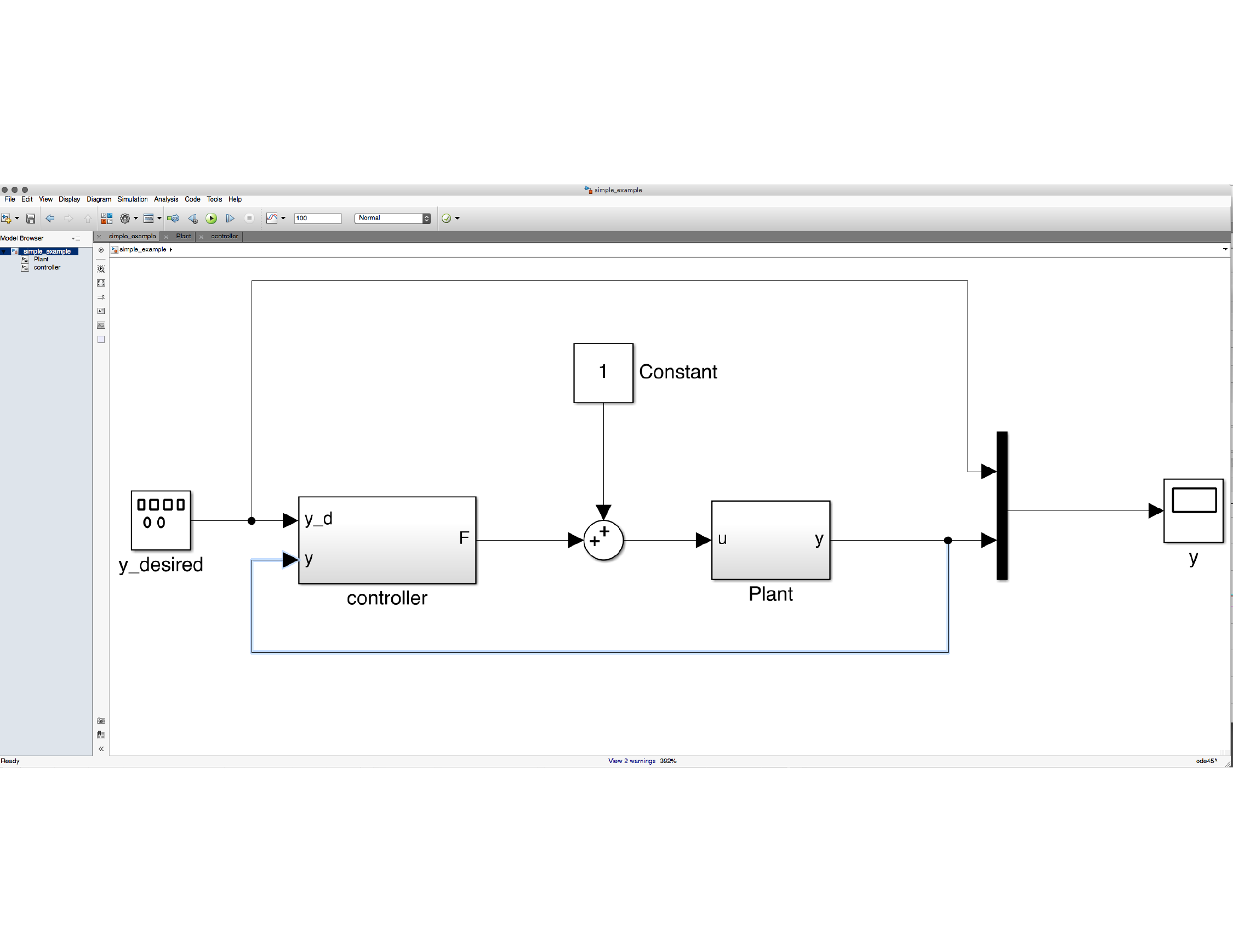
Consider the example in Sections 14.2.1, 15.2.1, and 16.2.1. A block diagram for the system is shown in Fig. 14.2, where a constant input disturbance has been added to the system.

Figure 14.2. Block diagram for a simple example, where a constant input disturbance has been added to the system.

Suppose that a standard feedback controller without an integrator and without a disturbance observer is designed for this system. An example of potential Python code is

import numpy as np
import control as cnt

P.A = np.array([[0., 1.0], [2.0, 3.0]])
P.B = np.array([[0.], [4.0]])
P.C = np.array([[5.0, 0]])
P.D = 0

P.Ts = 0.01 #sampling time

# pick poles for the controller
wn_ctrl = 1
zeta_ctrl = 0.707
charpoly = [1., 2.0*zeta_ctrl*wn_ctrl, wn_ctrl**2]
des_ctrl_poles = np.roots(charpoly)

# pick poles for the observer
wn_obsv = 10.0
zeta_obsv = 0.707
charpoly = [1., 2.0*zeta_obsv*wn_obsv, wn_obsv**2]
des_obsv_poles = np.roots(charpoly)

# is the system controllable?
    if np.linalg.matrix_rank(cnt.ctrb(P.A, P.B)) != np.size(P.A, 1):
print('System Not Controllable')
else:
    P.K = cnt.place(P.A, P.B, des_ctrl_poles)
    P.kr = -1.0/(P.C*np.linalg.inv(P.A-P.B*P.K)*P.B)

# is the system observable?
if np.linalg.matrix_rank(cnt.obsv(P.A, P.C)) != np.size(P.A, 1):
    print('System Not Observable')
else:
    P.L = cnt.place(P.A.T, P.C.T, des_obsv_poles).T

The associated control code is

# variables 'xhat' and 'u' must be declared as global, or
# class member variables for the sake of persistence, and the
# measurement 'y' and reference input 'r' must be passed in.
N = 10

# solve the observer differential equations using N steps of
# RK1 for i = 1 to N
for i in range(N):
    self.xhat = self.xhat + P.Ts/N*(P.A*self.xhat + \
                                    P.B*self.u + \
                                    P.L*(y-P.C*self.xhat))

# observer-based update with feedback controller
self.u = P.kr*r - P.K*self.xhat

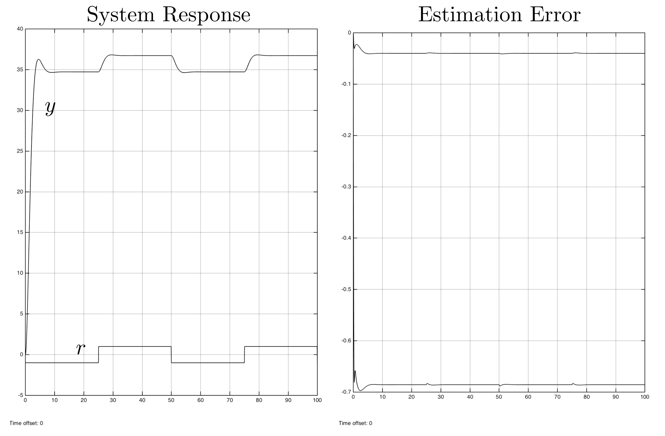
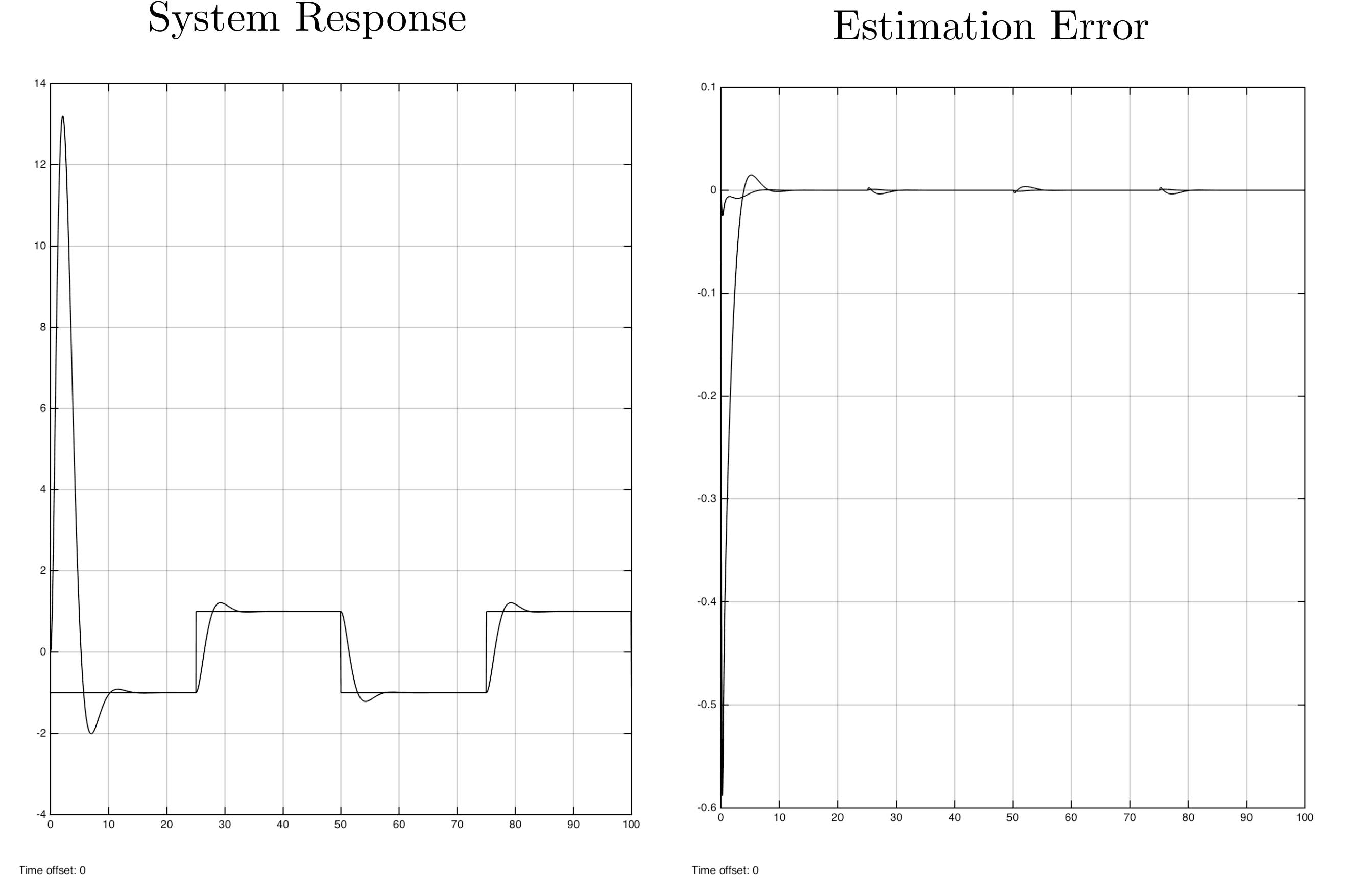
The step response for this controller is shown in Fig. 14.3, where it is obvious that the input disturbance is causing a large steady-state error in the system response, as well as in the estimation error.

Figure 14.3. Step response for standard observer-based control without integrator and without disturbance observer.

Figure 14.3 (Interactive). Adjust disturbance and reference to see steady-state and estimation-error behavior.

If an integrator is added to the system using the following design file

# design file with integrator
integrator_pole = -1.0

# augment system to add integrator
P.A1 = np.block([[P.A, np.zeros((2,1))], [-P.C, 0]])
P.B1 = np.block([[P.B], [0]])

# is this system controllable?
if np.linalg.matrix_rank(cnt.ctrb(P.A1, P.B1)) != np.size(P.A1, 1):
    print('System Not Controllable')
else:
    K1 = cnt.place(P.A1, P.B1, np.concatenate((des_ctrl_poles,
                                               [integrator_pole])))
    P.K = K1[0,0:-1]
    P.ki = K1[0, -1]

and the control code listed below:

# variables 'xhat,' 'error_d1, 'integrator,' and 'u' must be
# declared as global, or class member variables for the sake
# of persistence, and the measurement 'y' and reference input
# 'r' must be passed in.
N = 10

# solve the observer differential equations using N steps of
# RK1 for i = 1 to N
for i in range(N):
    self.xhat = self.xhat + P.Ts/N*(P.A*self.xhat + \
                                    P.B*self.u + \
                                    P.L*(y-P.C*self.xhat))

# implement the integrator
error = r-y
self.integrator = self.integrator + \
                  (P.Ts/2.0)*(error+self.error_d1)
self.error_d1 = error

# observer-based feedback controller
self.u = -P.K*self.xhat - P.ki*self.integrator

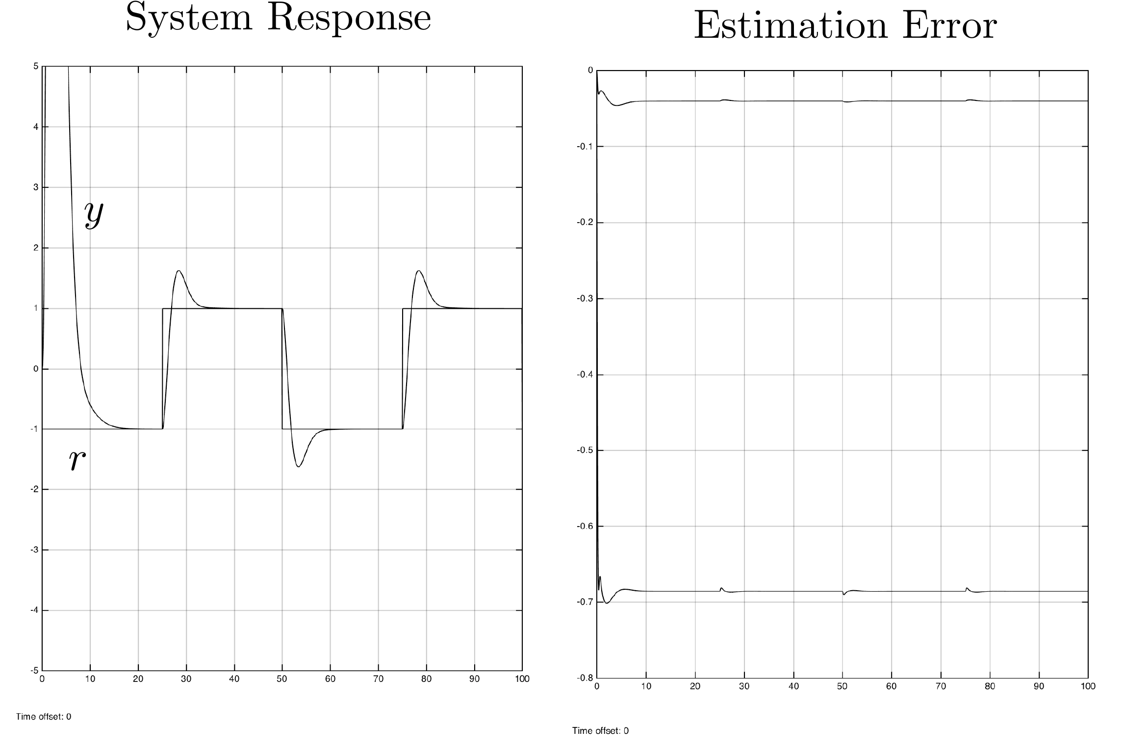
The response of the system with the integrator is shown in Fig. 14.4, where it is clear that the steady-state error in the response has been removed, but where there is now a steady-state response in the estimation error.

Figure 14.4. Step response for observer-based control with integrator but without disturbance observer.

Figure 14.4 (Interactive). Adjust disturbance and integrator gain to see tracking and estimation-error tradeoffs.

Now consider the case where the integrator is not present, but we add a disturbance observer. The design code is listed below.

# is the system controllable?
if np.linalg.matrix_rank(cnt.ctrb(P.A, P.B)) != np.size(P.A, 1):
    print('System Not Controllable')
else:
    P.K = cnt.place(P.A, P.B, des_ctrl_poles)
    P.kr = -1.0/(P.C*np.linalg.inv(P.A-P.B*P.K)*P.B)

# augment system for disturbance observer
disturb_obsv_pole = -2.0
P.A2 = np.block([[P.A, P.B], [np.zeros((1,2)), 0]])
P.B2 = np.block([[P.B], [0]])
P.C2 = np.block([P.C, 0])

# is the system observable?
if np.linalg.matrix_rank(cnt.obsv(P.A2, P.C2)) != np.size(P.A2, 1):
    print('System Not Observable')
else:
    P.L2 = cnt.place(P.A2.T, P.C2.T,
                     np.concatenate((des_obsv_poles,
                                     [disturb_obsv_pole]))).T

The associated control code is listed below.

# variables 'x_obsv' and 'u' must be declared as global, or
# class member variables for the sake of persistence, and the
# measurement 'y' and reference input 'r' must be passed in.
N = 10

# solve the observer differential equations using N steps of
# RK1 for i = 1 to N
for i in range(N):
    self.x_obsv = self.x_obsv + P.Ts/N*(P.A2*self.x_obsv + \
                                        P.B2*self.u + \
                                        P.L2*(y-P.C2*self.x_obsv))
xhat = self.x_obsv[0, 0:-1]
dhat = self.x_obsv[0, -1]

# observer-based feedback controller with disturbance observer
self.u = P.kr*r - P.K*self.xhat - dhat

Note the presence of \(\hat{d}\) on Line 13. The disturbance estimate is subtracted from the control input on Line 16. The resulting system response is shown in Fig. 14.5.

Figure 14.5. Step response for observer-based control with a disturbance observer rather than an integrator.

Figure 14.5 (Interactive). Adjust disturbance and disturbance-observer gain to compare disturbance rejection.

Note that in this case, the steady-state error in both the system response and the estimation error has been removed. At this point, the integrator can be added back into the system to remove the effect of model mismatch and other disturbances on the system.

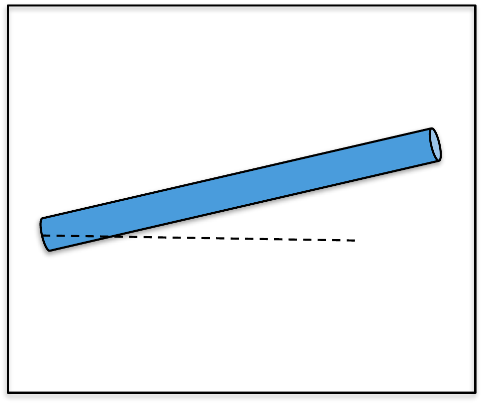
14.2 Design Study A. Single Link Robot Arm

14.2.1 Example Problem 3.1.17

(a) Modify the simulation from HW 3.1.16 so that the uncertainty parameter in arm_dynamics.m is \(\alpha=0.2\), representing 20% inaccuracy in the knowledge of the system parameters and so that the input disturbance is \(0.5\) Newton-meters. Also, add noise to the output channel \(\theta_m\) with a standard deviation of \(0.001\). Before adding the disturbance observer, run the simulation and note that the controller is not robust enough to handle the large input disturbance.

(b) Add a disturbance observer to the controller, and verify that the steady-state error in the estimator has been removed. Tune the system to get good response.

Design Study A guided exercise

Add a disturbance observer

Augment the observer so it estimates a constant input disturbance along with the plant state.

Step 1. Disturbance model

Constant disturbance derivative

Step 2. Augmented observer order

Number of estimated states

Step 3. Purpose

What should improve?

Pseudocode

The complete solution includes a simulation script and a disturbance-observer controller class. Before opening it, outline each component separately.

These prompts are ungraded. They are intended to connect the disturbance-observer design to the implementation code in the complete solution.

Complete solution

The single link robot arm is simulated using the following Python code.

# 3rd-party
import numpy as np

# local (controlbook)
import case_studies.A_arm.params as P
from case_studies.A_arm.dynamics import ArmDynamics
from case_studies.A_arm.ssi_dist_obs_controller import ArmSSIDOController
from case_studies.A_arm.visualizer import ArmVisualizer
from case_studies.common.signal_generator import SignalGenerator
from case_studies.common.simulation import run_simulation


arm = ArmDynamics(alpha=0.2)
controller = ArmSSIDOController(separate_integrator=False)
theta_ref = SignalGenerator(amplitude=np.radians(50), frequency=0.05)
d_force = np.array([0.5])
theta_noise = SignalGenerator(amplitude=0.001)

time, x_hist, u_hist, r_hist, xhat_hist, d_hist, dhat_hist = run_simulation(
    arm,
    [theta_ref],
    controller,
    controller_input="measurement",
    input_disturbance=d_force,
    output_noise=[theta_noise],
    t_final=20,
    dt=P.ts,
)

viz = ArmVisualizer(time, x_hist, u_hist, r_hist, xhat_hist, d_hist, dhat_hist)
viz.plot()
# viz.animate()

Note that in this simulation, the uncertainty parameter is \(\alpha=0.2\) implying \(20%\) variation in the plant parameters, and that the noise and disturbance are not zero.

A Python class that implements observer-based control with an integrator and disturbance observer for the single link robot arm is shown below.

# 3rd-party
import numpy as np
import control as cnt

# local (controlbook)
from . import params as P
from ..common.controller_base import ControllerBase


class ArmSSIDOController(ControllerBase):
    def __init__(self, separate_integrator=True):
        # control tuning parameters
        tr = 0.489
        zeta = 0.707
        integrator_pole = [-5.0]

        # augmented system
        A1 = np.block([[P.A, np.zeros((2, 1))], [-P.Cr, np.zeros(1)]])
        B1 = np.vstack((P.B, 0))

        # check controllability
        if np.linalg.matrix_rank(cnt.ctrb(A1, B1)) != 3:
            raise ValueError("System not controllable")

        # compute control gains
        wn = 2.2 / tr  # assumes zeta = 0.707
        des_char_poly = [1, 2 * zeta * wn, wn**2]
        des_sys_poles = np.roots(des_char_poly)
        des_poles = np.hstack((des_sys_poles, integrator_pole))
        self.K1 = cnt.place(A1, B1, des_poles)
        self.K = self.K1[:, :2]
        self.ki = self.K1[:, 2:]

        # linearization point
        self.x_eq = P.x_eq
        self.r_eq = P.Cr @ self.x_eq
        self.x1_eq = np.hstack((self.x_eq, 0))

        # integrator variables
        self.error_prev = 0.0
        self.error_integral = 0.0
        self.separate_integrator = separate_integrator

        ####### OBSERVER DESIGN ########
        # observer tuning parameters
        M_obs = 10.0  # time scale separation between controller and observer
        tr_obs = tr / M_obs
        zeta_obs = 0.707
        disturbance_pole = [-5.0]

        # augmented system
        self.A2 = np.block([[P.A, P.B], [np.zeros((1, 3))]])
        self.B2 = np.block([[P.B], [np.zeros(1)]])
        self.C2 = np.block([P.Cm, np.zeros(1)])

        # check observability
        if np.linalg.matrix_rank(cnt.ctrb(self.A2.T, self.C2.T)) != 3:
            raise ValueError("System not observable")

        # compute observer gain matrix
        wn_obs = 2.2 / tr_obs
        obs_char_poly = [1, 2 * zeta_obs * wn_obs, wn_obs**2]
        obs_sys_poles = np.roots(obs_char_poly)
        obs_poles = np.hstack((obs_sys_poles, disturbance_pole))
        self.L2 = cnt.place(self.A2.T, self.C2.T, obs_poles).T
        print("L2^T:", self.L2.T)

        # observer variables
        self.x2hat_tilde = np.zeros(3)
        self.u_prev = np.zeros(1)
        self.x2_eq = np.hstack((self.x_eq, [0]))

    def update_with_state(self, r, x):
        raise NotImplementedError("This controller only uses measurement feedback.")

    def update_with_measurement(self, r, y):
        # update the observer with the measurement
        xhat, dhat = self.observer_rk4_step(y)

        x_tilde = xhat - self.x_eq

        # integrate error
        error = r - P.Cr @ xhat  # can also use tilde vars (eq subtracts out)
        self.error_integral += P.ts * (error + self.error_prev) / 2
        self.error_prev = error

        # compute feedback control
        if self.separate_integrator:
            u_tilde = -self.K @ x_tilde - self.ki @ self.error_integral
        else:
            x1_tilde = np.hstack((x_tilde, self.error_integral))
            u_tilde = -self.K1 @ x1_tilde

        # convert back to original variables (for feedback linearization)
        theta = xhat[0]
        u_fl = P.m * P.g * P.ell / 2 * np.cos(theta)
        # subtract the disturbance estimate to actively compensate for disturbances
        u_unsat = u_tilde + u_fl - dhat
        u = self.saturate(u_unsat, u_max=P.tau_max)

        # save the previous control input for the observer
        self.u_prev = u

        return u, xhat, dhat

    def observer_f(self, x2hat_tilde, y):
        x2hat = x2hat_tilde + self.x2_eq
        y_error = y - self.C2 @ x2hat  # can also use tilde vars (eq subtracts out)
        u_fl = P.m * P.g * P.ell / 2 * np.cos(x2hat[0])
        u_tilde = self.u_prev - u_fl
        x2hat_dot = self.A2 @ x2hat_tilde + self.B2 @ u_tilde + self.L2 @ y_error
        return x2hat_dot

    def observer_rk4_step(self, y):
        k1 = self.observer_f(self.x2hat_tilde, y)
        k2 = self.observer_f(self.x2hat_tilde + P.ts / 2 * k1, y)
        k3 = self.observer_f(self.x2hat_tilde + P.ts / 2 * k2, y)
        k4 = self.observer_f(self.x2hat_tilde + P.ts * k3, y)
        x2hat_tilde_dot = (k1 + 2 * k2 + 2 * k3 + k4) / 6
        self.x2hat_tilde += x2hat_tilde_dot * P.ts

        # unpack estimated state and disturbance
        xhat_tilde = self.x2hat_tilde[:-1]
        xhat = xhat_tilde + self.x_eq
        dhat = self.x2hat_tilde[-1:]
        return xhat, dhat.copy()

Complete simulation code for MATLAB, Python, and Simulink can be downloaded at http://controlbook.byu.edu.

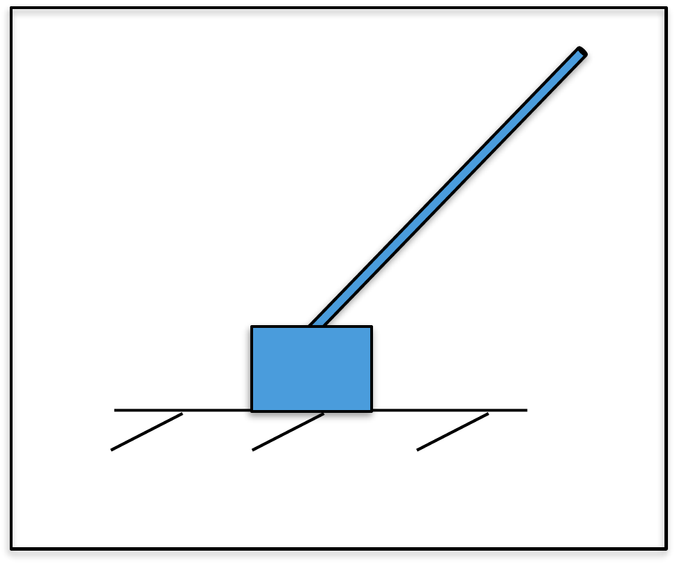
14.3 Design Study B. Inverted Pendulum

14.3.1 Example Problem 3.2.17

(a) Modify the simulation from HW 3.2.16 so that the uncertainty parameter in pendulum_dynamics.m is \(\alpha=0.2\), representing 20% inaccuracy in the knowledge of the system parameters, and so that the input disturbance is \(0.5\). Also, add noise to the output channels \(z_m\) and \(\theta_m\) with a standard deviation of \(0.001\). Before adding the disturbance observer, run the simulation and note that the controller is not robust to the large input disturbance.

(b) Add a disturbance observer to the controller, and verify that the steady-state error in the estimator has been removed. Tune the system to get good response.

Design Study B guided exercise

Add a disturbance observer

Augment the observer so it can estimate a constant input disturbance.

Step 1. Baseline failure mode

Observed problem

Step 2. Disturbance model

Disturbance derivative

Step 3. Noise level

Noise standard deviation

Pseudocode

The complete solution includes a simulation script and a disturbance-observer controller class. Before opening it, outline each component separately.

These prompts are ungraded. They are intended to connect the derivation to the implementation code in the complete solution.

Complete solution

The inverted pendulum is simulated using the following Python code.

# 3rd-party
import numpy as np

# local (controlbook)
import case_studies.B_pendulum.params as P
from case_studies.B_pendulum.dynamics import CartPendulumDynamics
from case_studies.B_pendulum.ssi_dist_obs_controller import CartPendulumSSIDOController
from case_studies.B_pendulum.visualizer import CartPendulumVisualizer
from case_studies.common.signal_generator import SignalGenerator
from case_studies.common.simulation import run_simulation


pendulum = CartPendulumDynamics(alpha=0.2)
controller = CartPendulumSSIDOController(separate_integrator=False)

z_ref = SignalGenerator(amplitude=0.5, frequency=0.04)
refs = [z_ref]

d_force = np.array([0.5])

z_noise = SignalGenerator(amplitude=0.001)
theta_noise = SignalGenerator(amplitude=0.001)
y_noise = [z_noise, theta_noise]

time, x_hist, u_hist, r_hist, xhat_hist, d_hist, dhat_hist = run_simulation(
    pendulum,
    refs,
    controller,
    controller_input="measurement",
    input_disturbance=d_force,
    output_noise=y_noise,
    t_final=60,
    dt=P.ts,
)

viz = CartPendulumVisualizer(time, x_hist, u_hist, r_hist, xhat_hist, d_hist, dhat_hist)
viz.plot()
# viz.animate()

Note that in this simulation, the uncertainty parameter is \(\alpha=0.2\) implying \(20%\) variation in the plant parameters, and that the noise and disturbance are not zero.

A Python class that implements observer-based control with an integrator and disturbance observer for the inverted pendulum is shown below.

# 3rd-party
import numpy as np
import control as cnt

# local (controlbook)
from . import params as P
from ..common.controller_base import ControllerBase


class CartPendulumSSIDOController(ControllerBase):
    def __init__(self, separate_integrator=True):
        # tuning parameters
        tr_theta = 0.8  # tuned for slower, more stable response.
        # May be necessary due to initial value for theta (10 degrees).
        zeta_theta = 0.9
        M = 3
        tr_z = tr_theta * M
        zeta_z = 0.9
        integrator_pole = [-2.0]

        # augmented system
        A1 = np.block([[P.A, np.zeros((4, 1))], [-P.Cr, np.zeros(1)]])
        B1 = np.vstack((P.B, 0))

        # check controllability
        if np.linalg.matrix_rank(cnt.ctrb(A1, B1)) != 5:
            raise ValueError("System not controllable")

        # compute gains
        wn_theta = 0.5 * np.pi / (tr_theta * np.sqrt(1 - zeta_theta**2))
        theta_char_poly = [1, 2 * zeta_theta * wn_theta, wn_theta**2]
        theta_poles = np.roots(theta_char_poly)

        wn_z = 0.5 * np.pi / (tr_z * np.sqrt(1 - zeta_z**2))
        z_char_poly = [1, 2 * zeta_z * wn_z, wn_z**2]
        z_poles = np.roots(z_char_poly)

        des_poles = np.hstack([theta_poles, z_poles, integrator_pole])

        self.K1 = cnt.place(A1, B1, des_poles)
        self.K = self.K1[:, :4]
        self.ki = self.K1[:, 4:]

        # linearization point
        self.x_eq = P.x_eq
        self.r_eq = P.Cr @ self.x_eq
        self.u_eq = P.u_eq

        # integrator variables
        self.error_prev = 0.0
        self.error_integral = 0.0
        self.separate_integrator = separate_integrator

        ####### OBSERVER DESIGN ########
        # observer tuning parameters
        M_obs = 10.0  # time scale separation between controller and observer
        tr_theta_obs = tr_theta / M_obs
        zeta_theta_obs = 0.9
        tr_z_obs = tr_z / M_obs
        zeta_z_obs = 0.9
        disturbance_pole = [-1.0]

        # augmented system
        self.A2 = np.block([[P.A, P.B], [np.zeros((1, 5))]])
        self.B2 = np.block([[P.B], [np.zeros(1)]])
        self.C2 = np.block([P.Cm, np.zeros((2, 1))])

        # check observability
        if np.linalg.matrix_rank(cnt.ctrb(self.A2.T, self.C2.T)) != 5:
            raise ValueError("System not observable")

        # compute observer gain matrix
        wn_theta_obs = 2.2 / tr_theta_obs
        theta_obs_char_poly = [1, 2 * zeta_theta_obs * wn_theta_obs, wn_theta_obs**2]
        theta_obs_poles = np.roots(theta_obs_char_poly)

        wn_z_obs = 2.2 / tr_z_obs
        z_obs_char_poly = [1, 2 * zeta_z_obs * wn_z_obs, wn_z_obs**2]
        z_obs_poles = np.roots(z_obs_char_poly)

        obs_poles = np.hstack((theta_obs_poles, z_obs_poles, disturbance_pole))
        self.L2 = cnt.place(self.A2.T, self.C2.T, obs_poles).T
        print("L^T:", self.L2.T)

        # observer variables
        self.x2hat_tilde = np.zeros(5)
        self.u_prev = np.zeros(1)
        self.x2_eq = np.hstack((self.x_eq, [0]))

    def update_with_state(self, r, x):
        raise NotImplementedError("This controller only uses measurement feedback.")

    def update_with_measurement(self, r, y):
        # update the observer with the measurement
        xhat, dhat = self.observer_rk4_step(y)

        # convert to linearization (tilde) variables
        x_tilde = xhat - self.x_eq
        r_tilde = r - self.r_eq

        # integrate error
        error = r - P.Cr @ xhat  # can also use tilde vars (eq subtracts out)
        self.error_integral += P.ts * (error + self.error_prev) / 2
        self.error_prev = error

        # compute feedback control
        if self.separate_integrator:
            u_tilde = -self.K @ x_tilde - self.ki @ self.error_integral
        else:
            x1_tilde = np.hstack((x_tilde, self.error_integral))
            u_tilde = -self.K1 @ x1_tilde

        # convert back to original variables and compensate for the disturbance
        u_unsat = u_tilde + self.u_eq - dhat
        u = self.saturate(u_unsat, u_max=P.force_max)

        # save the previous control input for the observer
        self.u_prev = u

        return u, xhat, dhat

    def observer_f(self, x2hat_tilde, y):
        x2hat = x2hat_tilde + self.x2_eq
        y_error = y - self.C2 @ x2hat  # can also use tilde vars (eq subtracts out)
        u_tilde = self.u_prev - self.u_eq
        x2hat_dot = self.A2 @ x2hat_tilde + self.B2 @ u_tilde + self.L2 @ y_error
        return x2hat_dot

    def observer_rk4_step(self, y):
        k1 = self.observer_f(self.x2hat_tilde, y)
        k2 = self.observer_f(self.x2hat_tilde + P.ts / 2 * k1, y)
        k3 = self.observer_f(self.x2hat_tilde + P.ts / 2 * k2, y)
        k4 = self.observer_f(self.x2hat_tilde + P.ts * k3, y)
        x2hat_tilde_dot = (k1 + 2 * k2 + 2 * k3 + k4) / 6
        self.x2hat_tilde += x2hat_tilde_dot * P.ts

        # unpack the state and disturbance estimates
        xhat_tilde = self.x2hat_tilde[:-1]
        xhat = xhat_tilde + self.x_eq
        dhat = self.x2hat_tilde[-1:]
        return xhat, dhat.copy()

Complete simulation code for MATLAB, Python, and Simulink can be downloaded at http://controlbook.byu.edu.

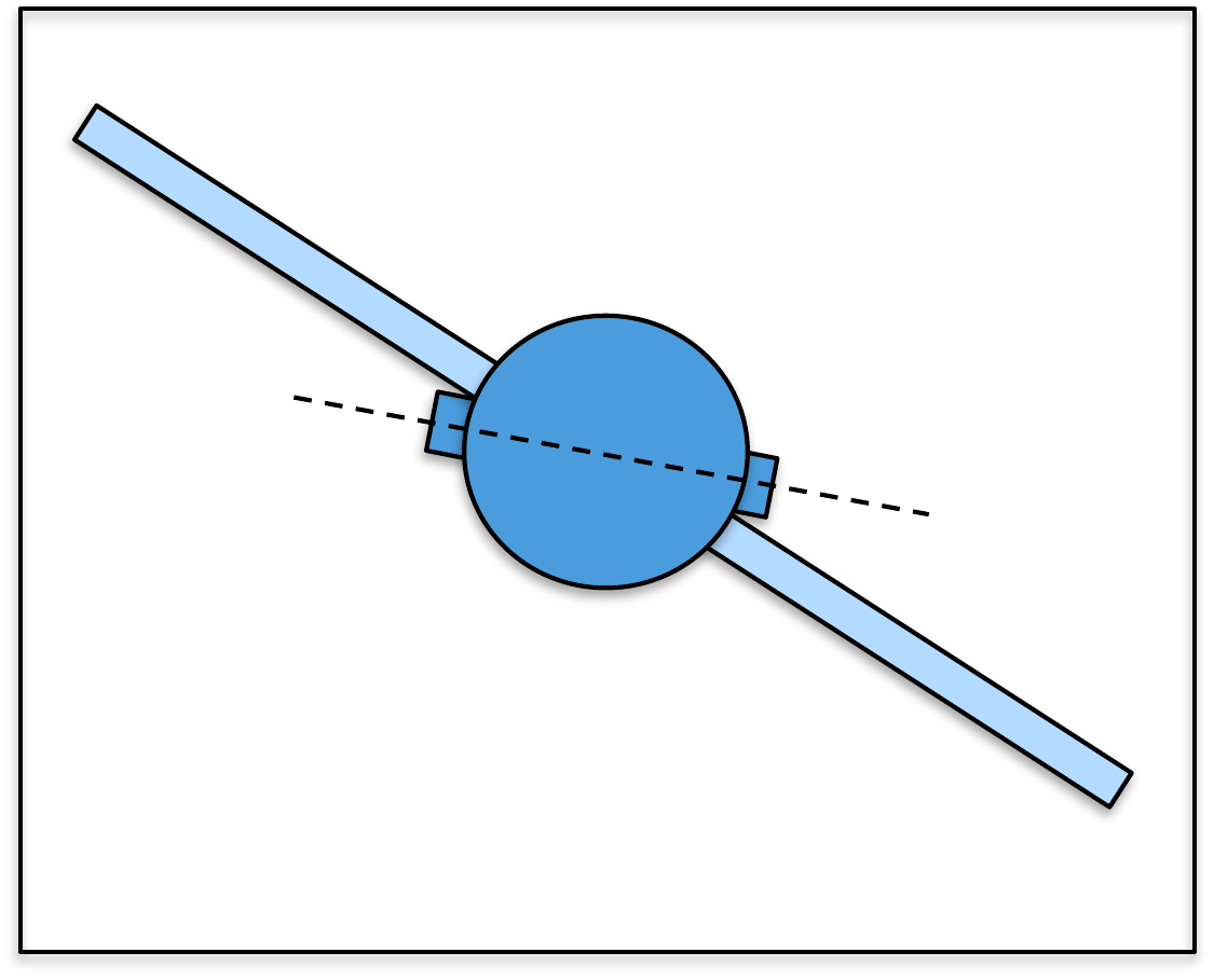
14.4 Design Study C. Satellite Attitude Control

14.4.1 Example Problem 3.3.17

(a) Modify the simulation from HW 3.3.16 so that the uncertainty parameter in satellite_dynamics.m is \(\alpha=0.2\), representing 20% inaccuracy in the knowledge of the system parameters and so that the input disturbance is \(1.0\) Newton-meters. Also, add noise to the output channels \(\phi_m\) and \(\theta_m\) with a standard deviation of \(0.001\). Before adding the disturbance observer, run the simulation and note that the controller is not robust to the large input disturbance.

(b) Add a disturbance observer to the controller, and verify that the steady-state error in the estimator has been removed. Tune the system to get good response.

Design Study C guided exercise

Plan the satellite disturbance observer

The disturbance observer estimates the input disturbance that the ordinary observer-based controller cannot reject robustly.

Step 1. Stress-test conditions

Uncertainty Measurement noise std.

Step 2. What gets estimated?

Extra estimated quantity Expected improvement

Pseudocode

Complete solution

The satellite is simulated using the following Python code.

# 3rd-party
import numpy as np

# local (controlbook)
import case_studies.C_satellite.params as P
from case_studies.C_satellite.dynamics import SatelliteDynamics
from case_studies.C_satellite.ssi_dist_obs_controller import SatelliteSSIDOController
from case_studies.C_satellite.visualizer import SatelliteVisualizer
from case_studies.common.signal_generator import SignalGenerator
from case_studies.common.simulation import run_simulation


satellite = SatelliteDynamics(alpha=0.2)
controller = SatelliteSSIDOController(separate_integrator=False)

phi_ref = SignalGenerator(amplitude=np.radians(15), frequency=0.015)
refs = [phi_ref]

d_torque = np.array([1.0])

theta_noise = SignalGenerator(amplitude=0.001)
phi_noise = SignalGenerator(amplitude=0.001)
y_noise = [theta_noise, phi_noise]

time, x_hist, u_hist, r_hist, xhat_hist, d_hist, dhat_hist = run_simulation(
    satellite,
    refs,
    controller,
    controller_input="measurement",
    input_disturbance=d_torque,
    output_noise=y_noise,
    t_final=100,
    dt=P.ts,
)

viz = SatelliteVisualizer(time, x_hist, u_hist, r_hist, xhat_hist, d_hist, dhat_hist)
viz.plot()
# viz.animate()

Note that in this simulation, the uncertainty parameter is \(\alpha=0.2\) implying \(20%\) variation in the plant parameters, and that the noise and disturbance are not zero.

A Python class that implements observer-based control with an integrator and disturbance observer for the satellite is shown below.

# 3rd-party
import numpy as np
import control as cnt

# local (controlbook)
from . import params as P
from ..common.controller_base import ControllerBase


class SatelliteSSIDOController(ControllerBase):
    def __init__(self, separate_integrator=False):
        # tuning parameters
        tr_theta = 2.0
        zeta_theta = 0.9
        M = 3  # time separation factor between inner and outer loop
        tr_phi = tr_theta * M
        zeta_phi = 0.9
        integrator_pole = [-1.0]

        # augmented system
        A1 = np.block([[P.A, np.zeros((4, 1))], [-P.Cr, np.zeros(1)]])
        B1 = np.vstack((P.B, 0))

        # check controllability
        if np.linalg.matrix_rank(cnt.ctrb(A1, B1)) != 5:
            raise ValueError("System not controllable")

        # compute gains
        wn_theta = 0.5 * np.pi / (tr_theta * np.sqrt(1 - zeta_theta**2))
        theta_char_poly = [1, 2 * zeta_theta * wn_theta, wn_theta**2]
        theta_poles = np.roots(theta_char_poly)

        wn_phi = 0.5 * np.pi / (tr_phi * np.sqrt(1 - zeta_phi**2))
        phi_char_poly = [1, 2 * zeta_phi * wn_phi, wn_phi**2]
        phi_poles = np.roots(phi_char_poly)

        des_poles = np.hstack([theta_poles, phi_poles, integrator_pole])

        self.K1 = cnt.place(A1, B1, des_poles)
        self.K = self.K1[:, :4]
        self.ki = self.K1[:, 4:]

        # linearization point
        self.x_eq = P.x_eq
        self.r_eq = P.Cr @ self.x_eq
        self.u_eq = P.u_eq

        # integrator variables
        self.error_prev = 0.0
        self.error_integral = 0.0
        self.separate_integrator = separate_integrator

        ####### OBSERVER DESIGN ########
        # observer tuning parameters
        M_obs = 10.0  # time scale separation between controller and observer
        tr_theta_obs = tr_theta / M_obs
        zeta_theta_obs = 0.9
        tr_phi_obs = tr_phi / M_obs
        phieta_phi_obs = 0.9
        disturbance_pole = [-1.0]

        # augmented system
        self.A2 = np.block([[P.A, P.B], [np.zeros((1, 5))]])
        self.B2 = np.block([[P.B], [np.zeros(1)]])
        self.C2 = np.block([P.Cm, np.zeros((2, 1))])

        # check observability
        if np.linalg.matrix_rank(cnt.ctrb(self.A2.T, self.C2.T)) != 5:
            raise ValueError("System not observable")

        # compute observer gain matrix
        wn_theta_obs = 2.2 / tr_theta_obs
        theta_obs_char_poly = [1, 2 * zeta_theta_obs * wn_theta_obs, wn_theta_obs**2]
        theta_obs_poles = np.roots(theta_obs_char_poly)

        wn_phi_obs = 2.2 / tr_phi_obs
        phi_obs_char_poly = [1, 2 * phieta_phi_obs * wn_phi_obs, wn_phi_obs**2]
        phi_obs_poles = np.roots(phi_obs_char_poly)

        obs_poles = np.hstack((theta_obs_poles, phi_obs_poles, disturbance_pole))
        self.L2 = cnt.place(self.A2.T, self.C2.T, obs_poles).T
        print("L^T:", self.L2.T)

        # observer variables
        self.x2hat_tilde = np.zeros(5)
        self.u_prev = np.zeros(1)
        self.x2_eq = np.hstack((self.x_eq, [0]))

    def update_with_state(self, r, x):
        raise NotImplementedError("This controller only uses measurement feedback.")

    def update_with_measurement(self, r, y):
        # update the observer with the measurement
        xhat, dhat = self.observer_rk4_step(y)

        # convert to linearization (tilde) variables
        x_tilde = xhat - self.x_eq
        r_tilde = r - self.r_eq

        # integrate error
        error = r - P.Cr @ xhat  # can also use tilde vars (eq subtracts out)
        self.error_integral += P.ts * (error + self.error_prev) / 2
        self.error_prev = error

        # compute feedback control
        if self.separate_integrator:
            u_tilde = -self.K @ x_tilde - self.ki @ self.error_integral
        else:
            x1_tilde = np.hstack((x_tilde, self.error_integral))
            u_tilde = -self.K1 @ x1_tilde

        # convert back to original variables and compensate for the disturbance
        u_unsat = u_tilde + self.u_eq - dhat
        u = self.saturate(u_unsat, u_max=P.torque_max)

        # save the previous control input for the observer
        self.u_prev = u

        return u, xhat, dhat

    def observer_f(self, x2hat_tilde, y):
        x2hat = x2hat_tilde + self.x2_eq
        y_error = y - self.C2 @ x2hat  # can also use tilde vars (eq subtracts out)
        u_tilde = self.u_prev - self.u_eq
        x2hat_dot = self.A2 @ x2hat_tilde + self.B2 @ u_tilde + self.L2 @ y_error
        return x2hat_dot

    def observer_rk4_step(self, y):
        k1 = self.observer_f(self.x2hat_tilde, y)
        k2 = self.observer_f(self.x2hat_tilde + P.ts / 2 * k1, y)
        k3 = self.observer_f(self.x2hat_tilde + P.ts / 2 * k2, y)
        k4 = self.observer_f(self.x2hat_tilde + P.ts * k3, y)
        x2hat_tilde_dot = (k1 + 2 * k2 + 2 * k3 + k4) / 6
        self.x2hat_tilde += x2hat_tilde_dot * P.ts

        # separate state and disturbance estimates
        xhat_tilde = self.x2hat_tilde[:-1]
        xhat = xhat_tilde + self.x_eq
        dhat = self.x2hat_tilde[-1:]
        return xhat, dhat.copy()

Simulation code for MATLAB, Python, and Simulink can be downloaded at http://controlbook.byu.edu.

14.5 Interactive Disturbance-Observer Check

Chapter 14 activity

Augmented disturbance-observer explorer

The plant receives a step to a constant input disturbance at t = 1 s. Change the disturbance size and the disturbance-observer pole to see how the augmented observer drives d toward the true disturbance through the innovation term y - Cx.

Reference command Constant input disturbance Disturbance-observer pole magnitude Final disturbance estimate Final tracking error Estimate settling time Interpretation

The same plant, controller, and augmented observer structure used in the chapter example are simulated. The pole slider moves the added disturbance-estimator pole.

For the matched constant-disturbance model, changing the pole should mainly change how quickly d converges. It should not be interpreted as changing the ideal final disturbance value.

Chapter 14 comparison

Standard observer vs. disturbance observer

Compare the standard observer-based controller with the augmented disturbance observer. Both see the same constant input disturbance, but only the augmented observer estimates d and subtracts it from the control input.

Reference command Constant input disturbance Disturbance-observer pole magnitude Standard final error Augmented final error Final d Main lesson

Dashed gray traces use the standard observer. Teal traces use the augmented disturbance observer. Dashed blue marks the reference command; dashed brown marks the true disturbance.

Chapter 14 code map

Connect the code to the observer equations

Select the mathematical role played by each line from the disturbance-observer implementation. The goal is to see how the code implements the augmented equations and the control input \(u = k_r r - K\hat{x} - \hat{d}\).

P.A2 = [[A, B], [0,
0]]

\(A_2 = \begin{bmatrix} A & B \\ 0 & 0 \end{bmatrix}\)

P.C2 = [C,
0]

\(C_2 = \begin{bmatrix} C & 0 \end{bmatrix}\)

y -
P.C2*x_obsv

\(y - C_2\hat{x}_2\)

dhat =
x_obsv[-1]

\(\hat{d} = \hat{x}_{2,\mathrm{last}}\)

u = kr*r - K*xhat -
dhat

\(u = k_r r - K\hat{x} - \hat{d}\) Correct matches Feedback

Chapter 14 observability

Can the augmented disturbance state be observed?

A disturbance observer augments the plant state with a constant-disturbance state, \(x_2 = [x_1,\;x_2,\;d]^T\). The observer can estimate \(d\) only when the augmented pair \((A_2, C_2)\) is observable.

Choose what the sensor measures through \(C\).
Choose where the disturbance enters through \(B_d\).
Check whether the resulting observability matrix has rank 3, which means both plant states and the added disturbance state can be inferred from output history.

Measured output Disturbance channel

Observability matrix

Rank

Interpretation

14.6 Knowledge Check

Q1. Disturbance observer purpose

A disturbance observer is intended to estimate:

A) Unknown disturbance effects B) Only the reference command C) Only sensor names D) No internal states

Q2. Model fit

A constant-disturbance observer is most useful when the disturbance is:

A) Persistent or slowly varying B) Pure measurement noise only C) Perfectly known already D) Infinite frequency

Q3. Augmented observer dimension

If a two-state plant is augmented with one constant-disturbance state, enter the observer model order.

Order:

Show solution

Answer: 3. The augmented observer estimates two plant states plus one disturbance state.

Q4. Bias reduction

If an output bias is 0.5 without disturbance estimation and 0.1 after estimation, enter the remaining bias.

Remaining bias:

Show solution

Answer: 0.1. The disturbance observer reduces the bias when the disturbance model matches the real disturbance.

Q5. Disturbance classification

Name one disturbance category discussed in the observer/disturbance chapters.

Answer:

Show solution

Answer: Examples include input disturbance, output disturbance, and model uncertainty.

Q6. Constant-disturbance augmentation

How is an unknown constant disturbance commonly represented in the augmented observer model?

A) As a state that must always equal zero. B) As a disturbance state with approximately zero derivative. C) As a state with infinite derivative. D) As a copy of the reference command.

Q7. Using the disturbance estimate

How should a disturbance estimate be used in the control law?

A) Only display it; never use it for compensation. B) Add it with an arbitrary sign, independent of where the disturbance enters. C) Replace the measured output with the disturbance estimate. D) Apply it through the correct modeled channel and sign to cancel the disturbance effect.

Q8. Poor model fit

Which disturbance is least well represented by a constant-disturbance observer?

A) A persistent output bias B) A slowly changing load C) A fast oscillatory, noise-like disturbance D) A constant torque bias

14.7 Notes and References

Disturbance observers are one example of how observers can be used to estimate a variety of different parameters in the system. In general, observers can be used to estimate model parameters like mass and inertia, but in this case, nonlinear observers are required. The most commonly used nonlinear observer is the extended Kalman filter. Derivations of the extended Kalman filter can be found in [24–26]. In robotics, observers are used to estimate the system state, but also the biases in gyroscopes and accelerometers [27], which are a form of input disturbances.