The root locus has been an important
pedagogical tool in control systems since the 1940s. It was important in
the design of feedback amplifiers for communication circuits where the
classic design involved the tuning of a small number of parameters. In
this appendix we introduce the root locus and show how it can be used to
understand the effect of adding an integrator to a second-order system
with PD control. However, we should note that root locus can be used in
many other settings. We are not including this appendix as a main
chapter in the book because in our experience root locus is rarely used
for actual design.
P.6.1 Theory
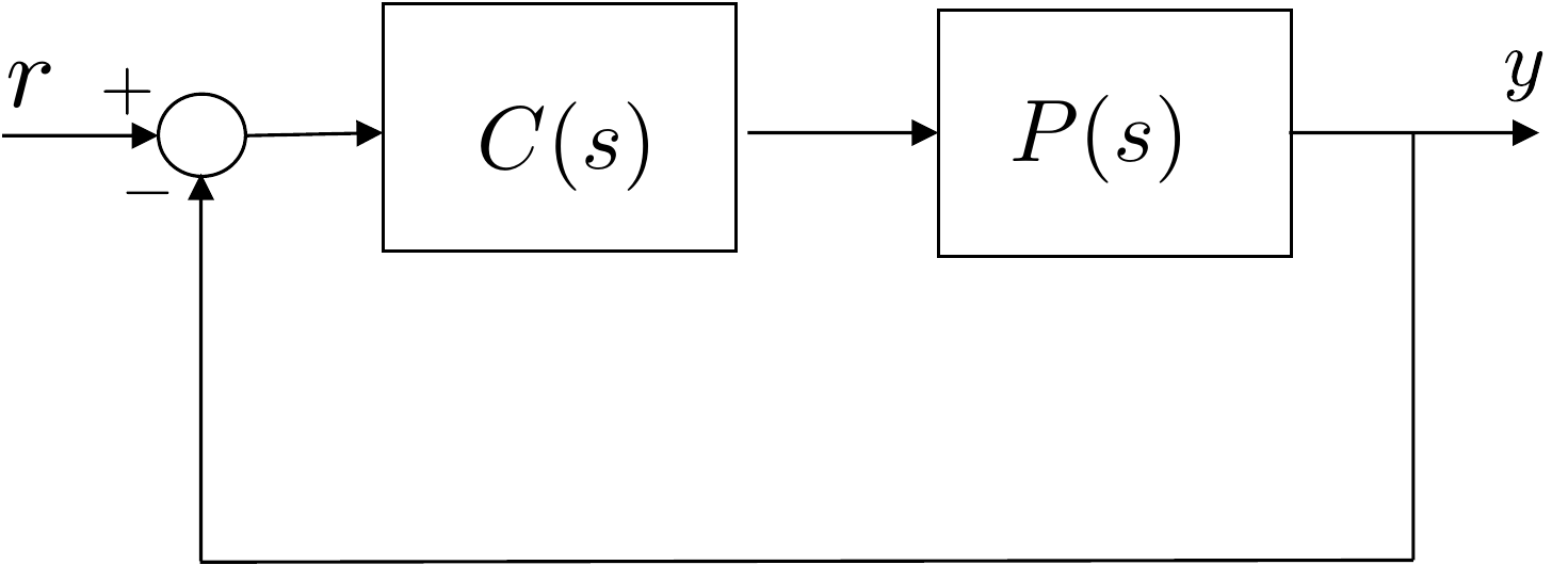
We begin by noting that for the closed-loop system shown in
Figure 6.1, the transfer
function from \(Y_r(s)\) to \(Y(s)\) can be computed as \[\begin{aligned}
&Y(s) = P(s)C(s)(Y_r(s)-Y(s)) \\
\implies & Y(s) = \frac{P(s)C(s)}{1+P(s)C(s)}Y_r(s).
\end{aligned}\] Therefore, the characteristic equation of the
closed-loop system is given by \[\Delta_{cl}
= 1+P(s)C(s)=0.\]
General feedback system with plant P(s) and controller C(s).
We have seen in
Chapter 10 that by using PD control
for a second-order system, it is possible to precisely select the
locations of the closed-loop poles. When an integrator is added for PID
control, it is also possible to precisely select the location of the
three closed-loop poles. In this chapter we will introduce a simple and
convenient tool for visualizing how the closed-loop poles change as a
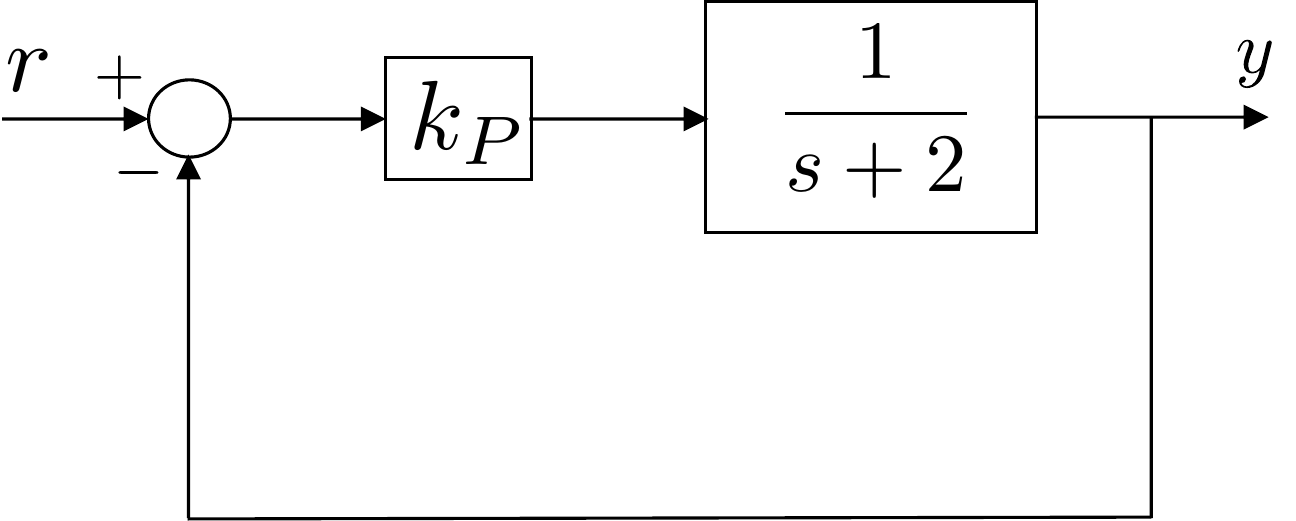
function of a single parameter. As motivation, consider a first-order
plant under proportional control, as shown in
Fig.6.2.
A first-order plant under proportional
control.
The closed-loop transfer function is given by \[Y(s) = \frac{k_P}{s+(2+k_P)} Y_r(s)\] and
the closed-loop characteristic polynomial is given by \[\Delta_{cl}(s) = s + (2+k_P).\] Note that
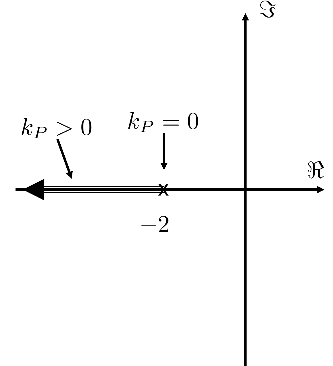
the location of the closed-loop pole is \[p_{cl} = -(2+k_P).\] We can create a plot
of the location of the poles in the complex plane as shown in
Fig.6.3.
A plot of the closed-loop pole associated
with Fig.6.2 as a function of
kP > 0.
When \(k_P=0\), the closed-loop pole
is located at the open-loop pole \(-2\), but as \(k_P\) is increased from zero, the
closed-loop pole moves from \(-2\) into
the left half-plane in the direction of the arrow shown in
Fig.6.3. The plot of the
closed-loop pole as a function of \(k_P\) is an example of a root
locus.
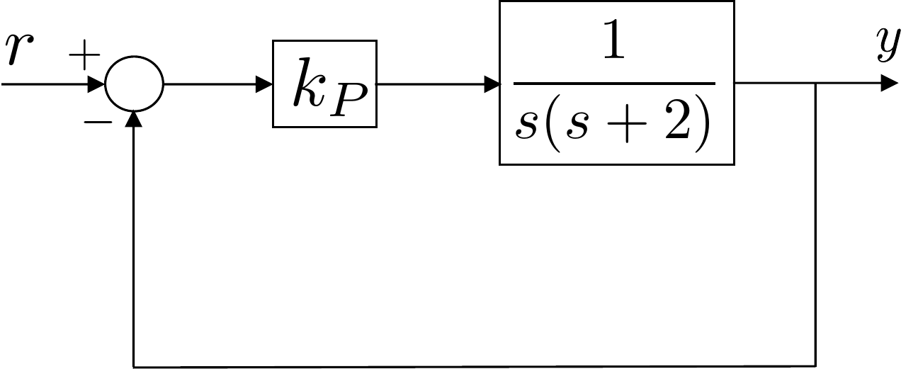
As a second example, consider the second-order system under
proportional control shown in
Fig.6.4.
A second-order plant under proportional
control.
In this case the closed-loop transfer function is given by \[Y(s) = \frac{k_P}{s^2+2s+k_P} Y_r(s)\]
Note that the open-loop poles are located at \(0\) and \(-2\). The closed-loop characteristic
polynomial is given by \[\tag{P.6.1}
\Delta_{cl}(s) = s^2 + 2s + k_P\] and the closed-loop poles are
located at \[p_{cl} = -1 \pm
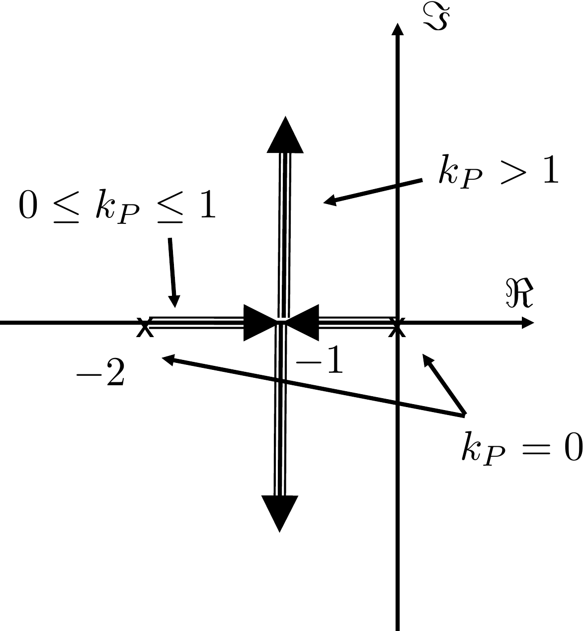
\sqrt{1-k_P}.\] The positions of the closed-loop poles as a
function of \(k_P>0\) are shown in
Fig.6.5.
A plot of the closed-loop poles
associated with Fig.6.4 as a function of
kP > 0.
When \(k_P=0\), the closed-loop
poles are equal to the open-loop poles at \(0\) and \(-2\). When \(0
< k_P \leq 1\), the closed-loop poles are both real and move
toward \(-1\) with increasing \(k_P\). When \(k_P=1\) both poles are located at \(-1\). When \(k_P>1\) the two poles are complex with
real part equal to \(-1\) and
increasing complex part as \(k_P\)
increases. The poles move in the direction of the arrows shown in
Fig.6.5.
The MATLAB command rlocus will plot the root locus and
can be used interactively to find the gain associated with specific pole
locations. To use the rlocus command in MATLAB, the
characteristic equation must be put in Evans’ form, which is
\[1 + kL(s) = 0,\] where \(k\) is the gain of interest. For example,
the characteristic equation associated with the characteristic
polynomial in
Equation P.6.1
is \[\Delta_{cl}(s) = s^2 + 2s + k_P =
0.\] The characteristic equation can be put in Evans’ form by
dividing both sides by \(s^2+2s\) and
rearranging to obtain \[1 +
k_P\left(\frac{1}{s^2+2s}\right) = 0,\] where \(L(s)=\frac{1}{s^2+2s}\). The MATLAB command
that draws the root locus for this equation is
where the first line defines the transfer function \(L(s)=\frac{1}{s^2+2s}\) and the second line
invokes the root locus command using \(L\).
The root locus tool is particularly useful for selecting the
integrator gains after PD gains
have been selected. For example, suppose that a PD controller has been
designed for the second-order plant shown in
Fig.6.6 so that the
closed-loop poles are located at \(-2\pm
j2\), where \(k_P=8\) and \(k_D=2\).
Closed loop system where the proportional
gains have been selected as kP = 8 and kD = 2.
Now suppose that an integrator is to be added to reject disturbances
and eliminate steady-state error, but that the integrator gain \(k_I\) is to be selected so that the
closed-loop poles deviate from \(-2\pm
j2\) by less than 10%. The characteristic equation for the
closed-loop system including the integrator is given by \[\begin{aligned}
&
1+\left(\frac{1}{s^2+2s}\right)\left(\frac{k_Ds^2+k_Ps+k_I}{s}\right) =
0 \\
\implies & \frac{(s^3 + 2s^2) + (k_Ds^2+k_Ps+k_I)}{s^3 + 2s^2} = 0
\\
\implies & s^3 + (2+k_D)s^2 + k_P s + k_I = 0 \\
\implies & \frac{(s^3 + (2+k_D)s^2 + k_P s) + k_I}{s^3 + (2+k_D)s^2
+ k_P s} = 0 \\
\implies & 1 + k_I\left(\frac{1}{s^3+(2+k_D)s^2+k_Ps}\right) = 0 \\
\implies & 1 + k_I\left(\frac{1}{s^3+4s^2+8s}\right)=0
\end{aligned}\] where the latter equation is in Evans’ form.
Therefore, the MATLAB command for drawing the root locus is
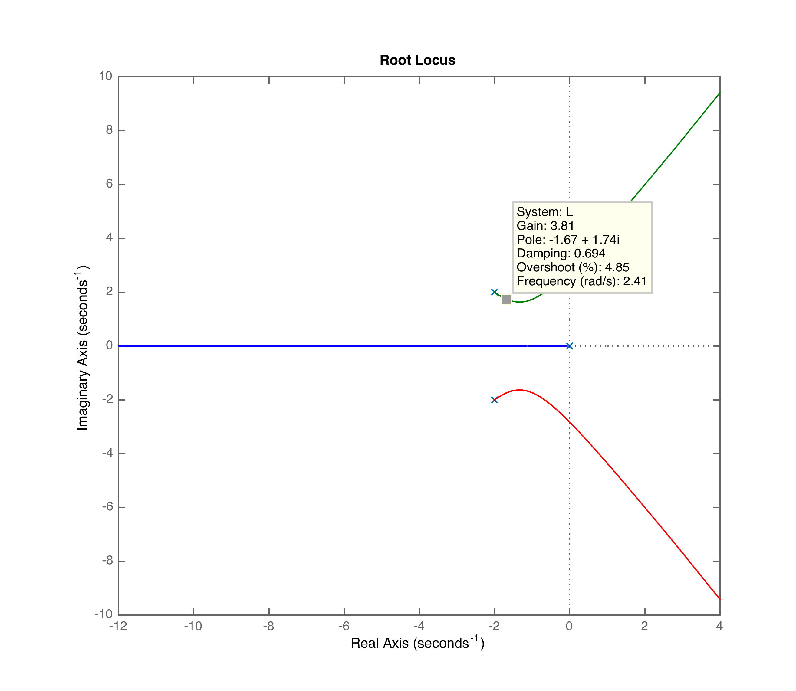
The result of MATLAB’s
rlocus command, with pole locations selected interactively
near −2 ± j2.
Note from
Fig.6.7 that the poles when
\(k_I=0\) are at \(0,-2\pm j2\) and are denoted by ‘x’. The
root locus shows what happens to the closed-loop poles as \(k_I\) is increased from zero. Note from
Fig.6.7 that for large values
of \(k_I\) the closed-loop poles are in
the right half-plane and the system will be unstable. However, for a
gain of \(k_I=3.81\) the closed-loop
poles are located at \(-1.67\pm
j1.74\). This technique can be used to select reasonable values
for \(k_I\).
For the single-link robot arm, use the PD gains derived in
HW 3.1.11. Add an integrator to the
controller to get PID control. Put the resulting closed-loop
characteristic equation in Evans’ form and use the MATLAB
rlocus command to plot the root locus versus the integrator
gain \(k_I\). Select a value for \(k_I\) that does not significantly change
the other locations of the closed-loop poles.
P.6.2.2 Solution
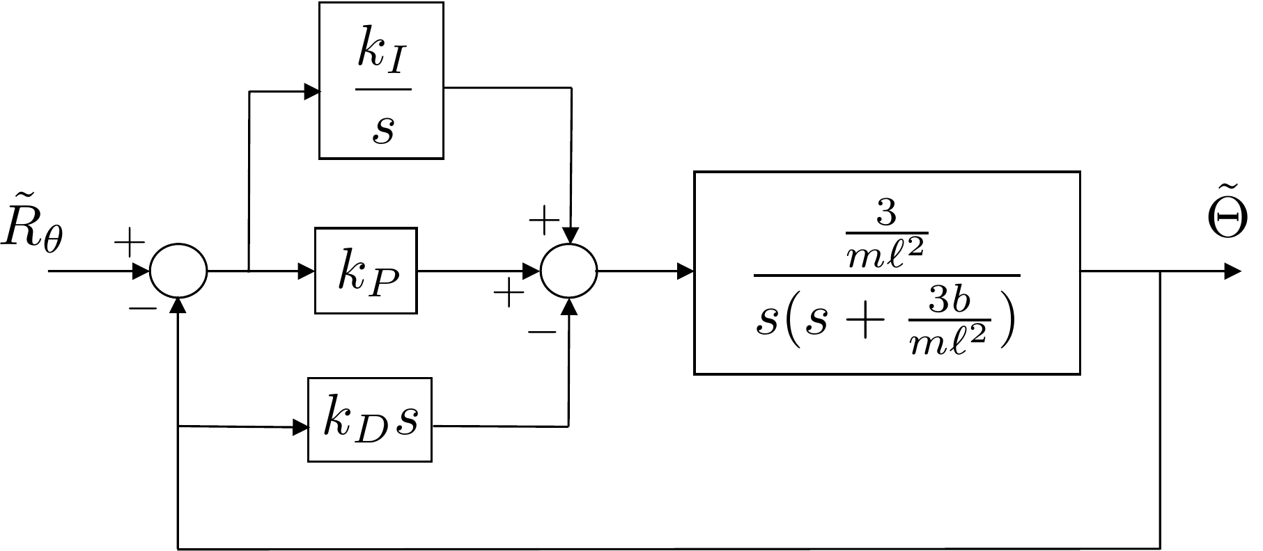
The closed-loop block diagram including an integrator is shown in
Fig.6.8.
PID control for the single-link robot
arm.
The closed-loop transfer function is given by \[\tilde{\Theta}(s) = \frac{\frac{3k_P}{m\ell^2}s +
\frac{3k_I}{m\ell^2}}{s^3 + \left(\frac{3b+3k_D}{m\ell^2}\right)s^2 +
\frac{3k_P}{m\ell^2}s + \frac{3k_I}{m\ell^2}}
\tilde{\Theta}^d(s).\] The characteristic equation is therefore
\[s^3 +
\left(\frac{3b+3k_D}{m\ell^2}\right)s^2 + \frac{3k_P}{m\ell^2}s +
\frac{3k_I}{m\ell^2} = 0.\] In Evans’ form we have \[1 + k_I\left(\frac{\frac{3}{m\ell^2}}{s^3 +
\left(\frac{3b+3k_D}{m\ell^2}\right)s^2 + \frac{3k_P}{m\ell^2}s}\right)
= 0.\] The appropriate MATLAB command is therefore
>> L = tf([3/m/L^2],...
          [1,(3*b+3*kd)/m/L^2,3*kp/m/L^2,0]);
>> figure(1), clf, rlocus(L);
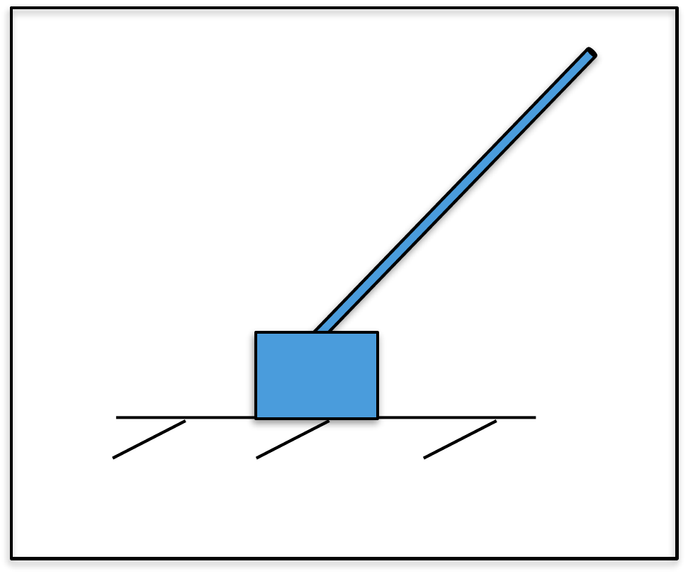
Add an integrator to obtain PID control for the outer loop of the
inverted pendulum system. Put the characteristic equation in Evans’ form
and use the MATLAB rlocus command to plot the root locus
versus the integrator gain \(k_I\).
Select a value for \(k_I\) that does
not significantly change the other locations of the closed-loop
poles.
Design
Study B guided exercise
Set up the pendulum root
locus
Put the outer-loop PID characteristic equation in
Evans form and vary the integral gain.
Use the block diagram to identify the
transfer function multiplied by k_I.
Step 1.
Root-locus gain
Show
solution for Step 1
Answer: The
root locus is plotted versus the integral gain k_I.
Step 2.
Evans form
Show
solution for Step 2
Answer: Evans
form is written as 1 + k_I L(s) = 0.
Step
3. Gain selection goal
Show solution for Step
3
Answer: Choose k_I so it does not
significantly move the existing dominant poles.
Pseudocode
The complete solution includes
implementation code. Before opening it, outline the algorithm in your
own words.
This prompt is ungraded. It is intended to
connect the derivation to the implementation code in the complete
solution.
Complete solution
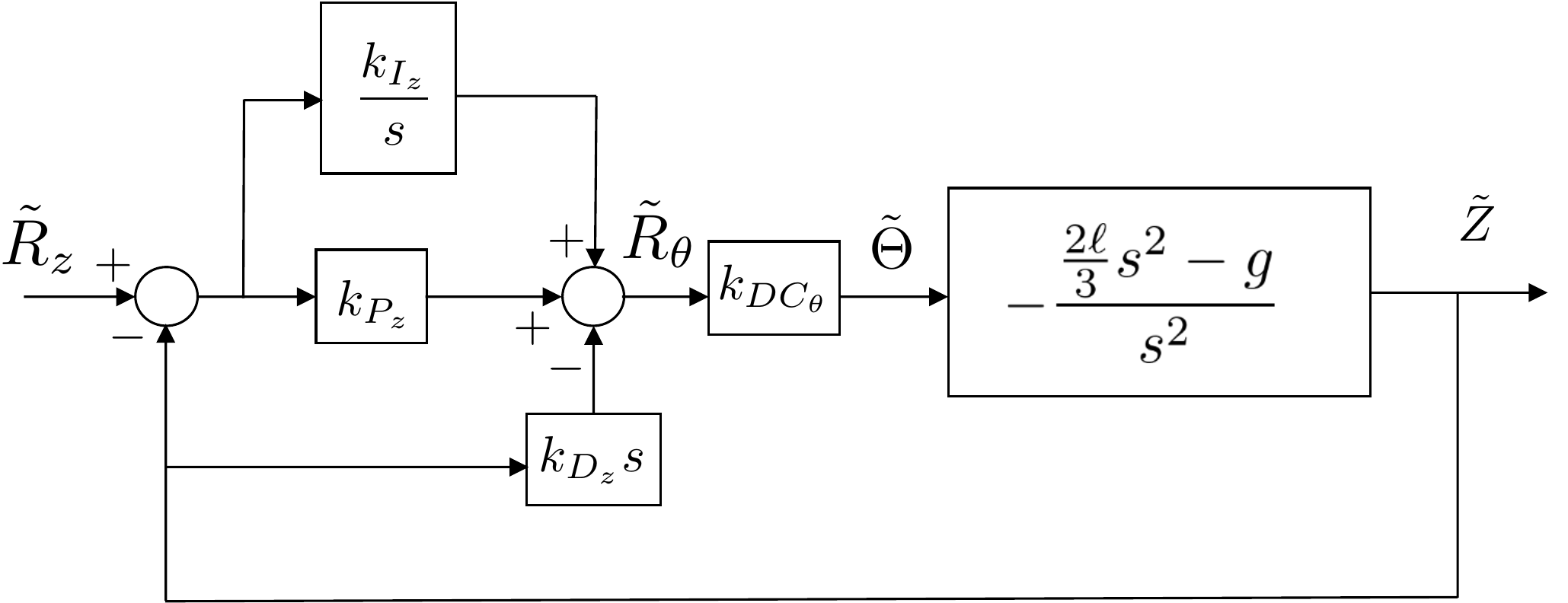
The closed-loop block diagram for the outer loop of the inverted
pendulum including an integrator is shown in Fig.6.9.
PID control for the outer loop of the
inverted pendulum.
The closed-loop transfer function is given by \[\tilde{Z}(s) = \frac{(g-\frac{2}{3}\ell s^2
)\left(k_{P_z}s+k_{I_z}\right)}{-\frac{2}{3}\ell k_{D_z} s^4 +
\left(\frac{1}{k_{DC_\theta}}-\frac{2}{3} \ell k_{P_z}\right)s^3 + (g
k_{D_z}-\frac{2}{3}\ell k_{I_z})s^2 + gk_{P_z}s + g k_{I_z}}
\tilde{Z}_r(s).\] The characteristic equation is therefore \[-\frac{2}{3}\ell k_{D_z} s^4 +
\left(\frac{1}{k_{DC_\theta}}-\frac{2}{3} \ell k_{P_z}\right)s^3 + (g
k_{D_z}-\frac{2}{3}\ell k_{I_z})s^2 + gk_{P_z}s + g k_{I_z} =
0.\] In Evans’ form we have \[1 +
k_{I_z}\left(\frac{-\frac{2}{3}\ell s^2+g}{-\frac{2}{3}\ell k_{D_z} s^4
+ \left(\frac{1}{k_{DC_\theta}}-\frac{2}{3} \ell k_{P_z}\right)s^3 + g
k_{D_z}s^2 + gk_{P_z}s}\right) = 0.\] The appropriate MATLAB
command is therefore
>> L = tf([-2/3*ell,0,g],...
          [-2/3*ell*kd,1/kDCth-2/3*ell*kp,g*kd,g*kp,0]);
>> figure(1), clf, rlocus(L);
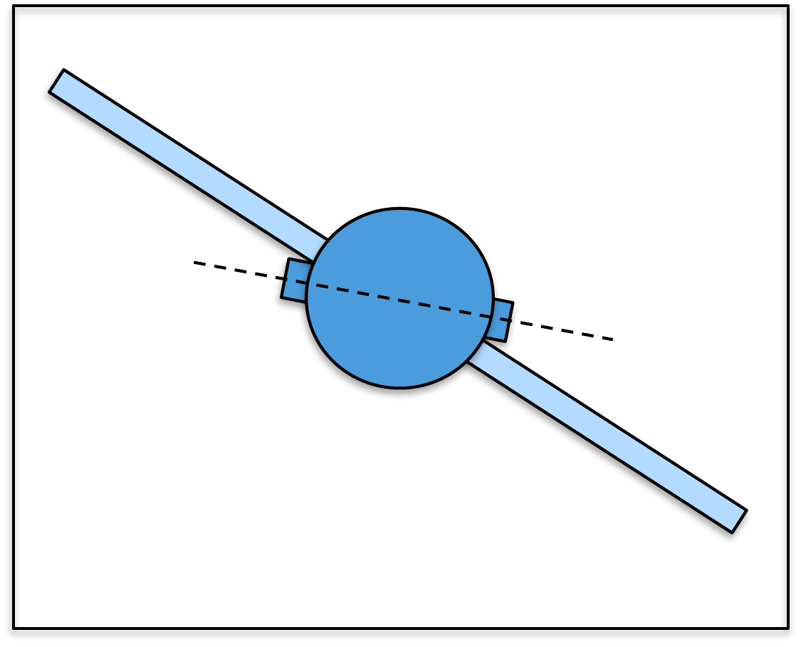
Add an integrator to obtain PID control for the outer loop of the
satellite system. Put the characteristic equation in Evans’ form and use
the MATLAB rlocus command to plot the root locus versus the
integrator gain \(k_I\). Select a value
for \(k_I\) that does not significantly
change the other locations of the closed-loop poles.
Design
Study C guided appendix
Interpret the satellite PID root
locus
The root-locus task adds an outer-loop integrator and
varies \(k_I\). The goal is to remove steady-state error without moving
the dominant poles too much.
Step 1. Root-locus gain
Show
solution for Step 1
Answer: The
varied root-locus gain is \(k_I\) for the outer loop.
Step 2. Gain-selection
criterion
Show solution for Step
2
Answer: Choose \(k_I\) so the
existing dominant poles do not move significantly; overly aggressive
integral action can reduce damping or excite flexible
motion.
Complete solution
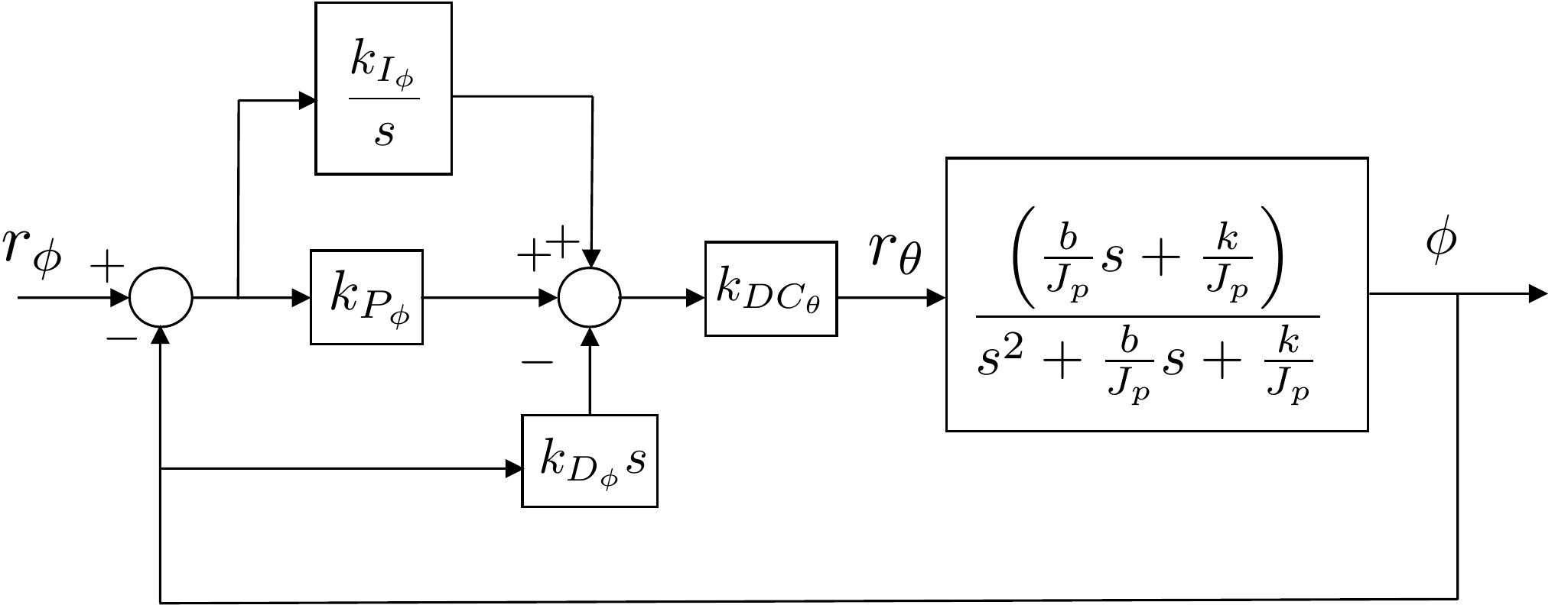
The closed-loop block diagram for the outer loop including an
integrator is shown in Fig.6.10.
PID control for the outer loop of the
satellite system.
The closed-loop transfer function is given by \[\Phi(s) = \frac{b_2s^2 + b_1 s +
b_0}{a_3s^3+a_2s^2+a_1s+a_0}\Phi_r(s),\] where \[\begin{aligned}
b_2 &=\frac{bk_{DC_\theta}k_{P_\phi}}{J_p} \\
b_1 &=
\frac{bk_{DC_\theta}k_{I_\phi}}{J_p}+\frac{kk_{DC_\theta}k_{P_\phi}}{J_p}
\\
b_0 &= \frac{kk_{DC_\theta}k_{I_\phi}}{J_p} \\
a_3 &= 1+\frac{bk_{DC_\theta}k_{D_\phi}}{J_p} \\
a_2 &=
\frac{b}{J_p}+\frac{kk_{DC_\theta}k_{D_\phi}}{J_p}+\frac{bk_{DC_\theta}k_{P_\phi}}{J_p}
\\
a_1 &=
\frac{k}{J_p}+\frac{bk_{DC_\theta}k_{I_\phi}}{J_p}+\frac{kk_{DC_\theta}k_{P_\phi}}{J_p}
\\
a_0 &= \frac{kk_{DC_\theta}k_{I_\phi}}{J_p}.
\end{aligned}\] The characteristic equation is therefore \[\begin{gathered}
\left(1+\frac{bk_{DC_\theta}k_{D_\phi}}{J_p}\right)s^3
+
\left(\frac{b}{J_p}+\frac{kk_{DC_\theta}k_{D_\phi}}{J_p}+\frac{bk_{DC_\theta}k_{P_\phi}}{J_p}\right)s^2
\\ +
\left(\frac{k}{J_p}+\frac{bk_{DC_\theta}k_{I_\phi}}{J_p}+\frac{kk_{DC_\theta}k_{P_\phi}}{J_p}\right)s
+ \frac{kk_{DC_\theta}k_{I_\phi}}{J_p} = 0.
\end{gathered}\] In Evans’ form we have \[1 +
k_{I_\phi}\left(\frac{\frac{bk_{DC_\theta}}{J_p}s+\frac{kk_{DC_\theta}}{J_p}}
{\left(1+\frac{bk_{DC_\theta}k_{D_\phi}}{J_p}\right)s^3 +
\left(\frac{b}{J_p}+\frac{kk_{DC_\theta}k_{D_\phi}}{J_p}+\frac{bk_{DC_\theta}k_{P_\phi}}{J_p}\right)s^2
+ \left(\frac{k}{J_p}+\frac{kk_{DC_\theta}k_{P_\phi}}{J_p}\right)s}
\right) = 0.\] The appropriate MATLAB command is therefore