To achieve the objectives discussed in
Chapter 19, the closed-loop
system must be stable. Recall that tracking performance and disturbance
rejection characteristics are
determined by the loop shape at low frequencies
when \(\left|P(j\omega)C(j\omega)\right|\gg
1\). Similarly, noise attenuation properties are
determined by the loop shape at high frequencies when \(\left|P(j\omega)C(j\omega)\right|\ll 1\).
In both cases we ignored the phase of \(P(j\omega)C(j\omega)\). It turns out that
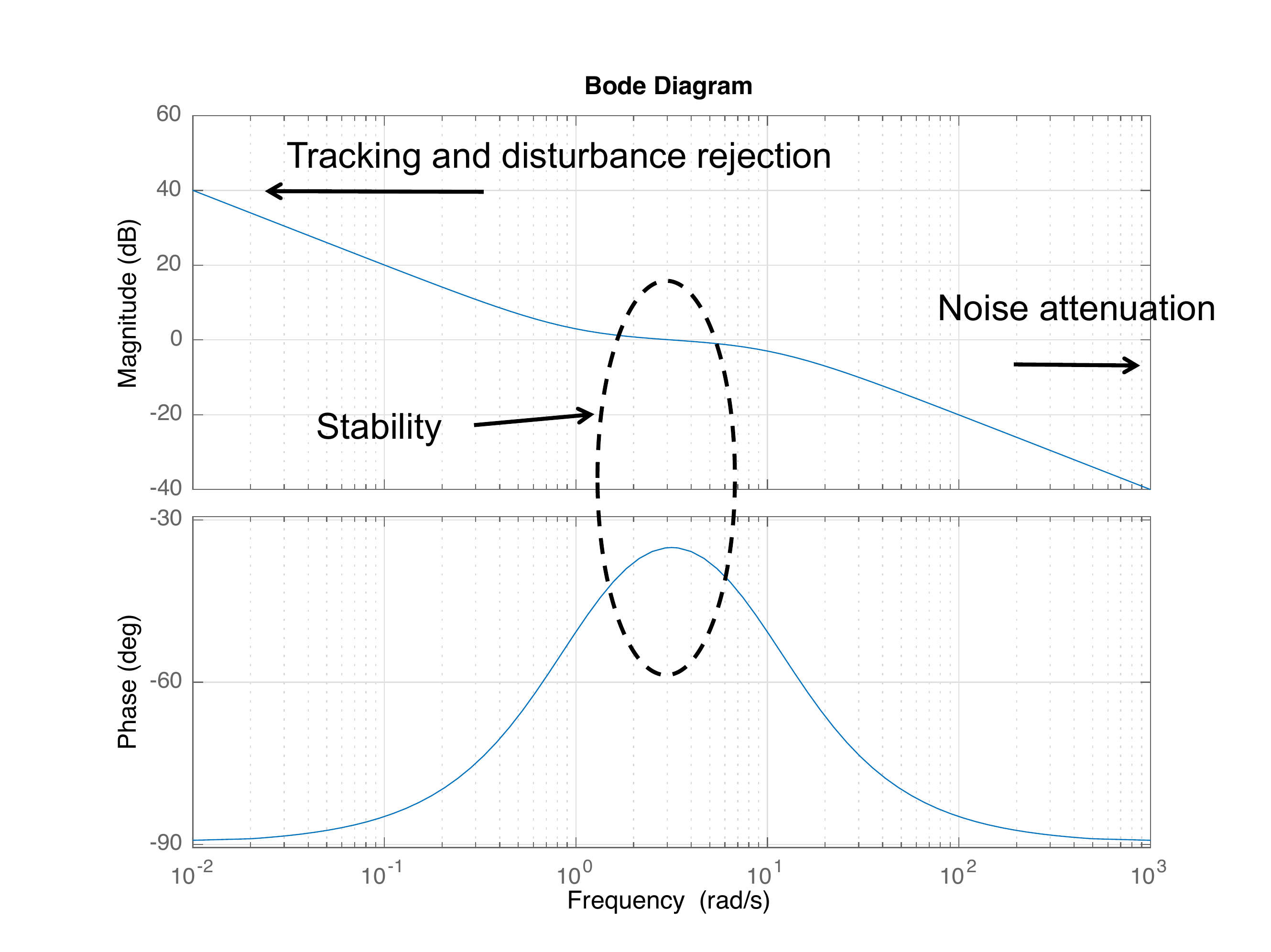
stability of the closed-loop system is determined by the phase of \(P(j\omega)C(j\omega)\) when \(P(j\omega)C(j\omega)=1\), as depicted in
Fig.17.1.
Figure 17.1. The shape of the magnitude plot primarily
determines the tracking and disturbance rejection characteristics at low
frequencies and the noise attenuation at high frequencies. Stability is
primarily determined by the phase at the crossover
frequency.
Define the crossover frequency \(\omega_{co}\) to be the frequency
where \[\left|P(j\omega_{co})C(j\omega_{co})\right|=1,\]
or equivalently where \[20\log_{10}\left|P(j\omega_{co})C(j\omega_{co})\right|
= 0\text{~dB}.\] The phase \(\angle
P(j\omega_{co})C(j\omega_{co})\) at the crossover frequency plays
a critical role in determining the stability of the system. To better
understand why this is the case, consider the transfer functions from
\(R\), \(D_{in}\), \(D_{out}\), and \(N\), to \(E\) in
Equation 16.3.
The denominator in each transfer function is \(1+P(s)C(s)\). Therefore, the closed-loop
poles are given by the closed-loop characteristic equation \[1+P(s)C(s) = 0,\] or equivalently where
\[P(s)C(s) = -1.\]
Recall that for any \(s\), \(P(s)C(s)\) is a complex number with
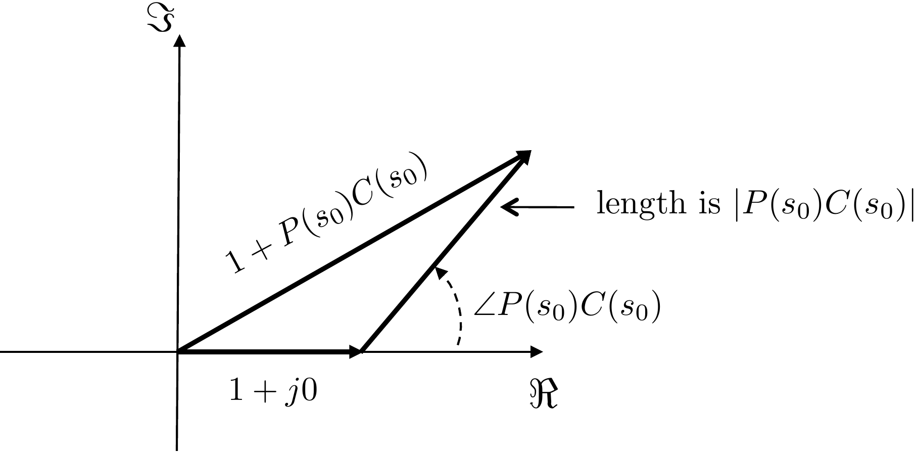
magnitude and phase. Therefore, given any \(s_0\) we can draw \(1+P(s_0)C(s_0)\) in the complex plane as
shown in
Fig.17.2.
Figure 17.2. The plot of 1 + P(s0)C(s0)
in the complex plane, is the sum of the complex number 1 + j0 and P(s0)C(s0).
Since the physical response of the system is determined by \(P(s)C(s)\) evaluated on the \(j\omega\)-axis, there are stability
problems if there exists an \(\omega_0\) such that \(P(j\omega_0)C(j\omega_0)=-1\), or in other
words when \[\left|P(j\omega_0)C(j\omega_0)\right|=1
\qquad\text{and}\qquad \angle P(j\omega_0)C(j\omega_0) =
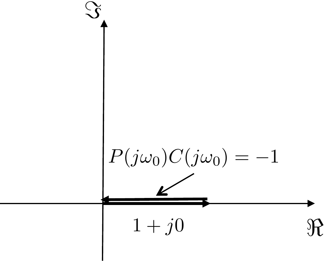
-180^\circ,\] as shown in
Fig.17.3.
Figure 17.3. The plot of 1 + P(jω0)C(jω0)
in the complex plane when P(jω0)C(jω0) = −1.
Since the magnitude of the loop gain is equal to one at the
crossover frequency \(\omega_{co}\), it
turns out that the quality of stability is determined by the phase of
the loop gain at the crossover frequency. Define the phase margin
\(PM\) as \[PM = \angle P(j\omega_{co})C(j\omega_{co}) -
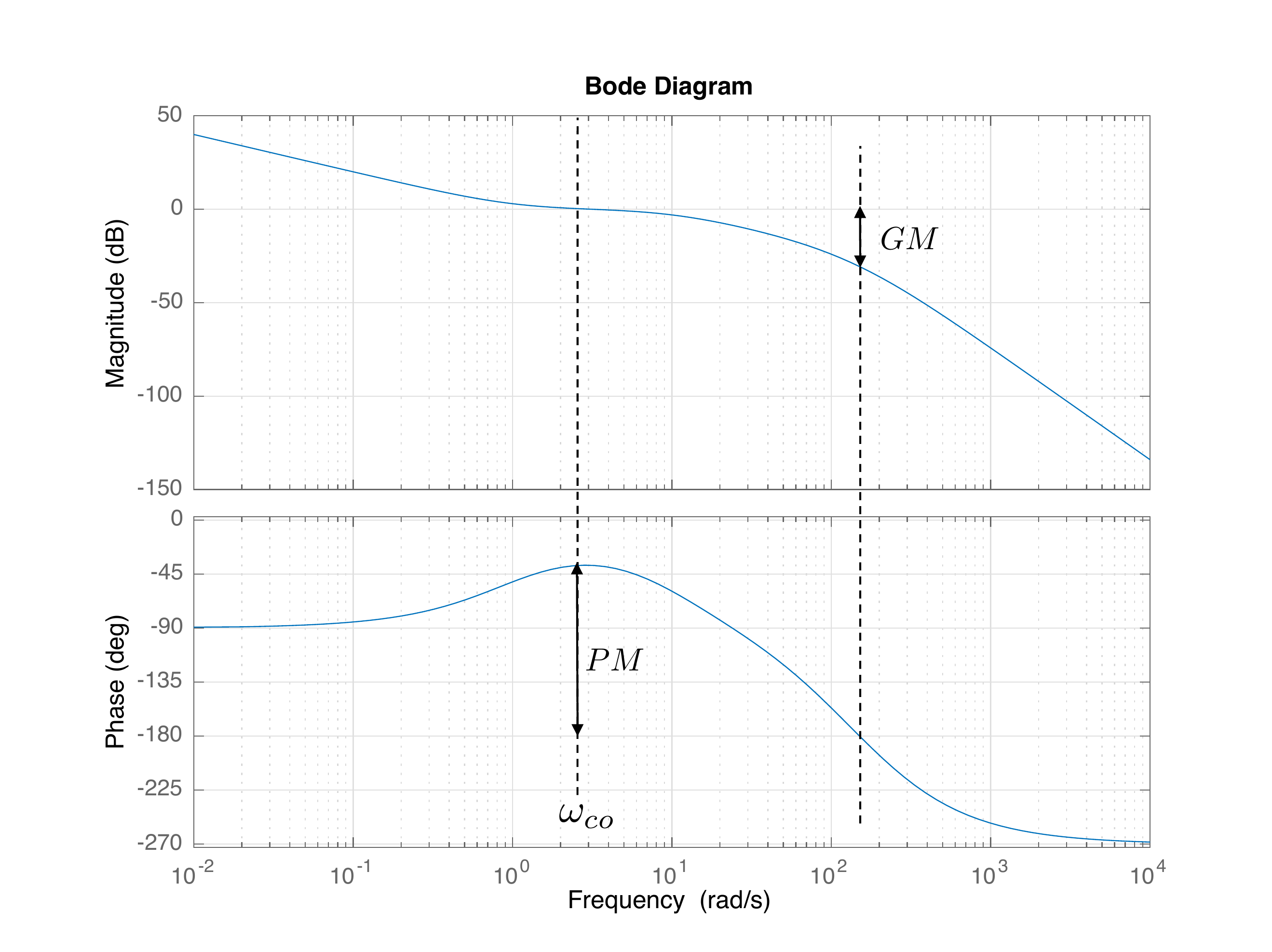
(-180)^\circ.\]Fig.17.4 depicts the phase margin on
the Bode plot.
Figure 17.4. The phase margin PM is the difference
between the phase of P(jω)C(jω)
and −180 degrees at the crossover
frequency ωco.
The gain margin GM is
the magnitude of P(jω)C(jω)
when the phase crosses −180 degrees.
Chapter 17 interactive figure
Measure gain and phase margins on a Bode plot
Move the
loop gain and added phase lag. The same loop shape is used in the gain
and phase plots, so the crossover markers and margin measurements update
together.
Increasing gain
usually moves the gain crossover. Adding phase lag directly reduces the
phase margin and can reduce the gain margin.
Figure 1.9. Interactive Figure 17.I1. Phase margin is read at
gain crossover; gain margin is read at phase crossover.
Gain crossover
Phase crossover
Phase margin
Gain margin
Robustness note
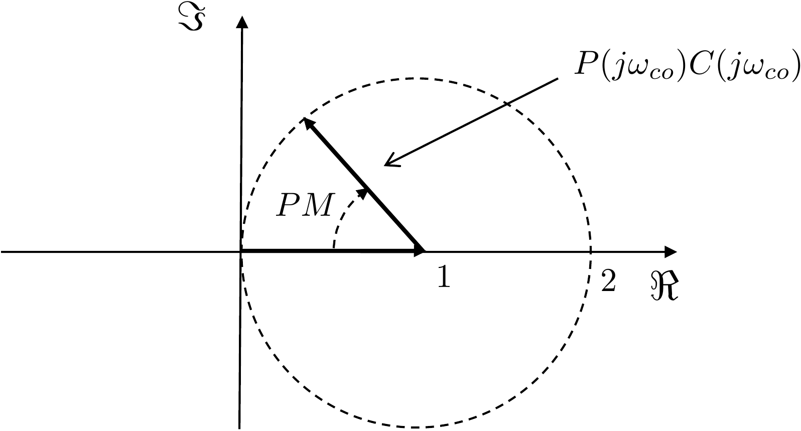
Another way to understand the phase margin is shown in
Fig.17.5. The phase margin indicates
the angular distance that \(P(j\omega_{co})C(j\omega_{co})\) is from
\(-1\).
Figure 17.5. Alternative graphical view of the phase
margin PM.
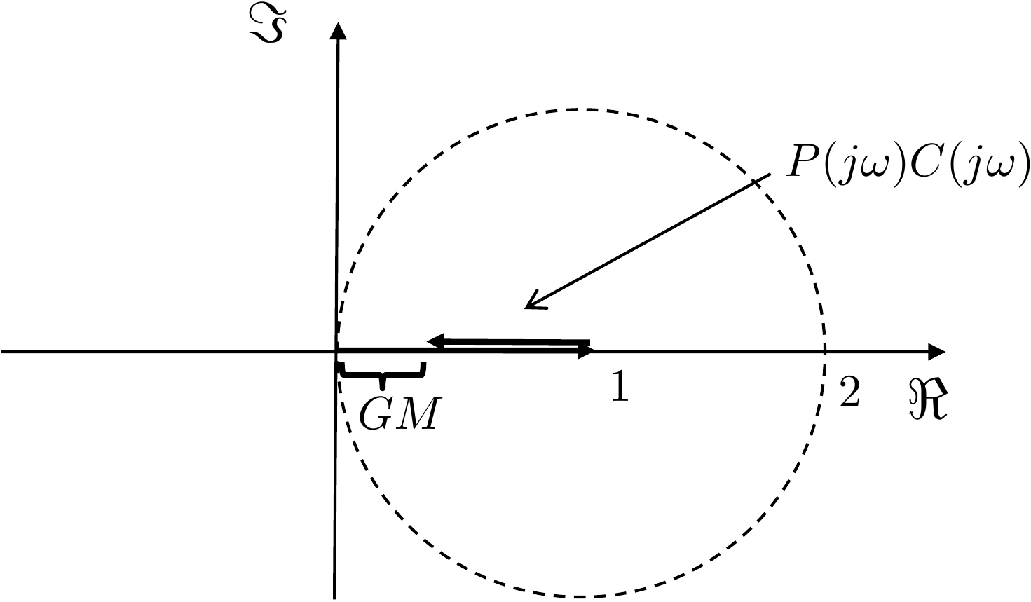
A related quantity is the Gain Margin \(GM\), which measures how far
the magnitude \(\left|P(j\omega)C(j\omega)\right|\) is from
unity when the phase \(\angle
P(j\omega)C(j\omega) = -180\) degrees. The gain margin is
depicted on the Bode plot in
Fig.17.4. An alternative view is shown
in
Fig.17.6.
Figure 17.6. Alternative graphical view of the gain
margin GM.
A good control design will have large phase and gain margins. A phase
margin of \(PM=60\) degrees is
considered to be very good and is optimal for many applications. A gain
margin of \(GM=10\) dB would be
considered very good for most applications.
17.1.2 Open and Closed Loop
Frequency Response
From
Equation 16.1,
the transfer function from the reference \(R(s)\) to the output \(Y(s)\) is \[Y(s)
= \frac{P(s)C(s)}{1+P(s)C(s)}R(s)\] Note that
when \(\left|P(j\omega)C(j\omega)\right|\gg 1\),
then \(\left|\frac{P(j\omega)C(j\omega)}{1+P(j\omega)C(j\omega)}\right|\approx
1\),
when \(\left|P(j\omega)C(j\omega)\right|\ll 1\),
then \(\left|\frac{P(j\omega)C(j\omega)}{1+P(j\omega)C(j\omega)}\right|\approx
\left|P(j\omega)C(j\omega)\right|\).
When \(\left|P(j\omega)C(j\omega)\right|=1\),
i.e., when \(\omega=\omega_{co}\), then
\(\left|\frac{P(j\omega_{co})C(j\omega_{co})}{1+P(j\omega_{co})C(j\omega_{co})}\right|\)
is a complex number divided by a complex number, and the magnitude will
depend on the phase of the \(P(j\omega_{co})C(j\omega_{co})\), or in
other words the phase margin \(PM\). As
shown in Figure 17.5, \(PM\) will determine the magnitude of \(1+P(j\omega_{co})C(j\omega_{co})\). When
\(PM\) is small, \(\left|1+P(j\omega_{co})C(j\omega_{co})\right|\)
will be small and \(\left|\frac{P(j\omega_{co})C(j\omega_{co})}{1+P(j\omega_{co})C(j\omega_{co})}\right|\)
will be larger than one. When \(PM\) is
larger than \(90\) degrees, \(\left|1+P(j\omega_{co})C(j\omega_{co})\right|\)
will be larger than \(\left|P(j\omega_{co})C(j\omega_{co})\right|\)
and \(\left|\frac{P(j\omega_{co})C(j\omega_{co})}{1+P(j\omega_{co})C(j\omega_{co})}\right|\)
will be less than one.
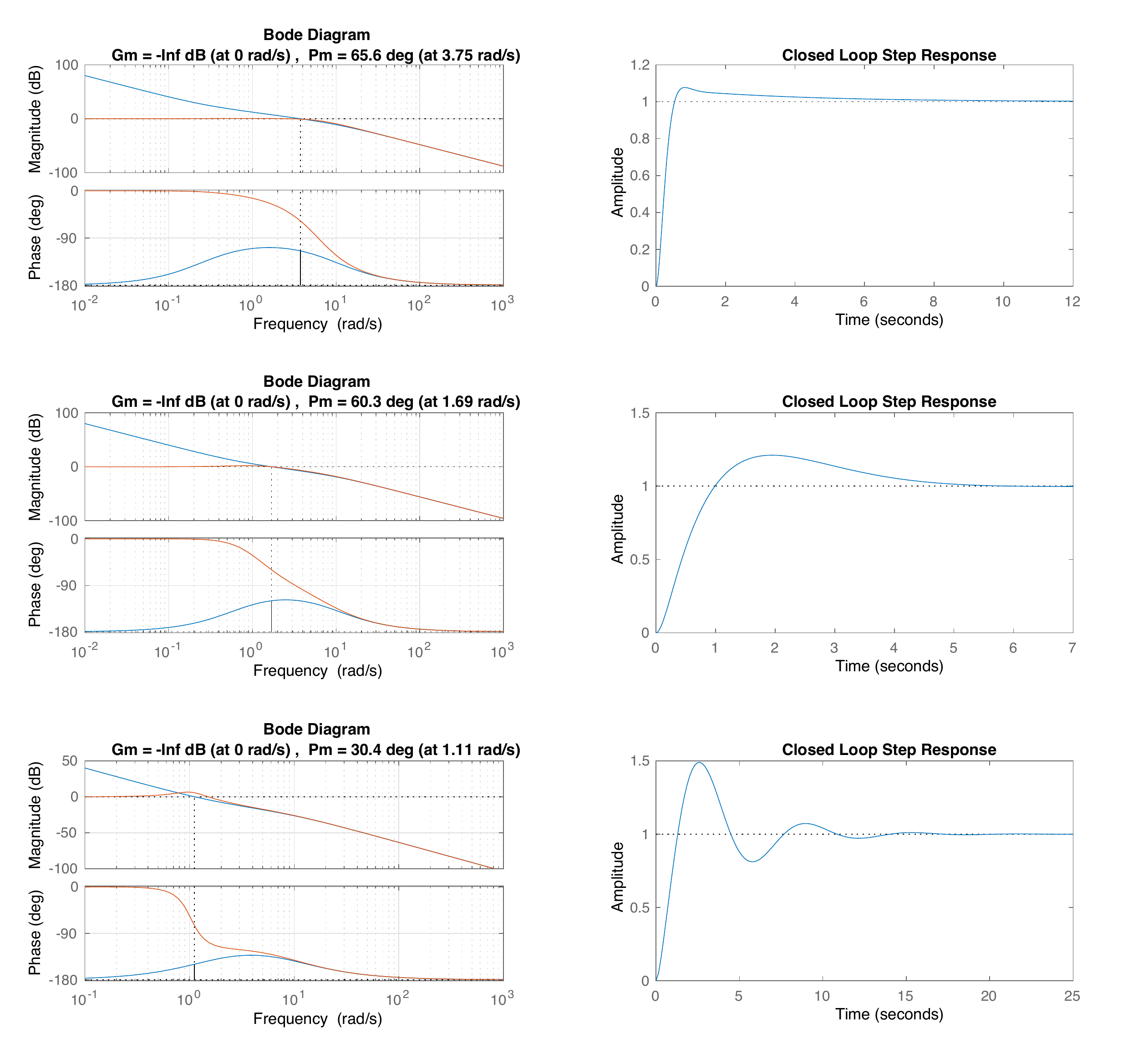
Fig.17.7 shows the
closed-loop Bode plot superimposed on the
open-loop Bode plot for different values of the phase margin. Note that
when the phase margin is \(PM=60\) degrees, the closed-loop frequency
response looks very similar to the closed-loop frequency response for a
second-order system when \(\zeta=0.707\), as shown in
Fig.15.9. Phase margins smaller
than \(60\) degrees have a peaking
response similar to a second-order system with \(\zeta<0.707\). Note also that the
bandwidth of the closed-loop system is approximately the crossover
frequency of the open-loop system. In general, the crossover frequency
\(\omega_{co}\) plays a similar role
for general systems that the natural frequency \(\omega_n\) plays for second-order systems.
Figure 17.7. Closed-loop Bode plot superimposed on the
open-loop Bode plot, together with the closed-loop step response, for
different phase margins.
Chapter 17 interactive figure
Phase margin, closed-loop peaking, and ringing
Predict
what will happen before moving the slider: if the phase margin
decreases, should the closed-loop frequency-response peak and the
step-response overshoot increase or decrease? The plots use a
second-order approximation to show the trend described in the
text.
Figure 1.10. Interactive Figure 17.I3. Smaller phase margin increases
the closed-loop resonant peak and step-response overshoot. Faint curves
show reference cases at 45, 60, and 80 degrees.
Damping proxy
Closed-loop peak
Step overshoot
Design
interpretation
Approximation used
Fig.17.7 also shows the
corresponding step response for the closed-loop system. The step response
looks similar to the step response for second-order systems shown in
Fig.8.3,
where again, the step response for \(PM=60\) degrees in
Fig.17.7 is roughly
equivalent to the step response for \(\zeta=0.707\) in
Fig.8.4.
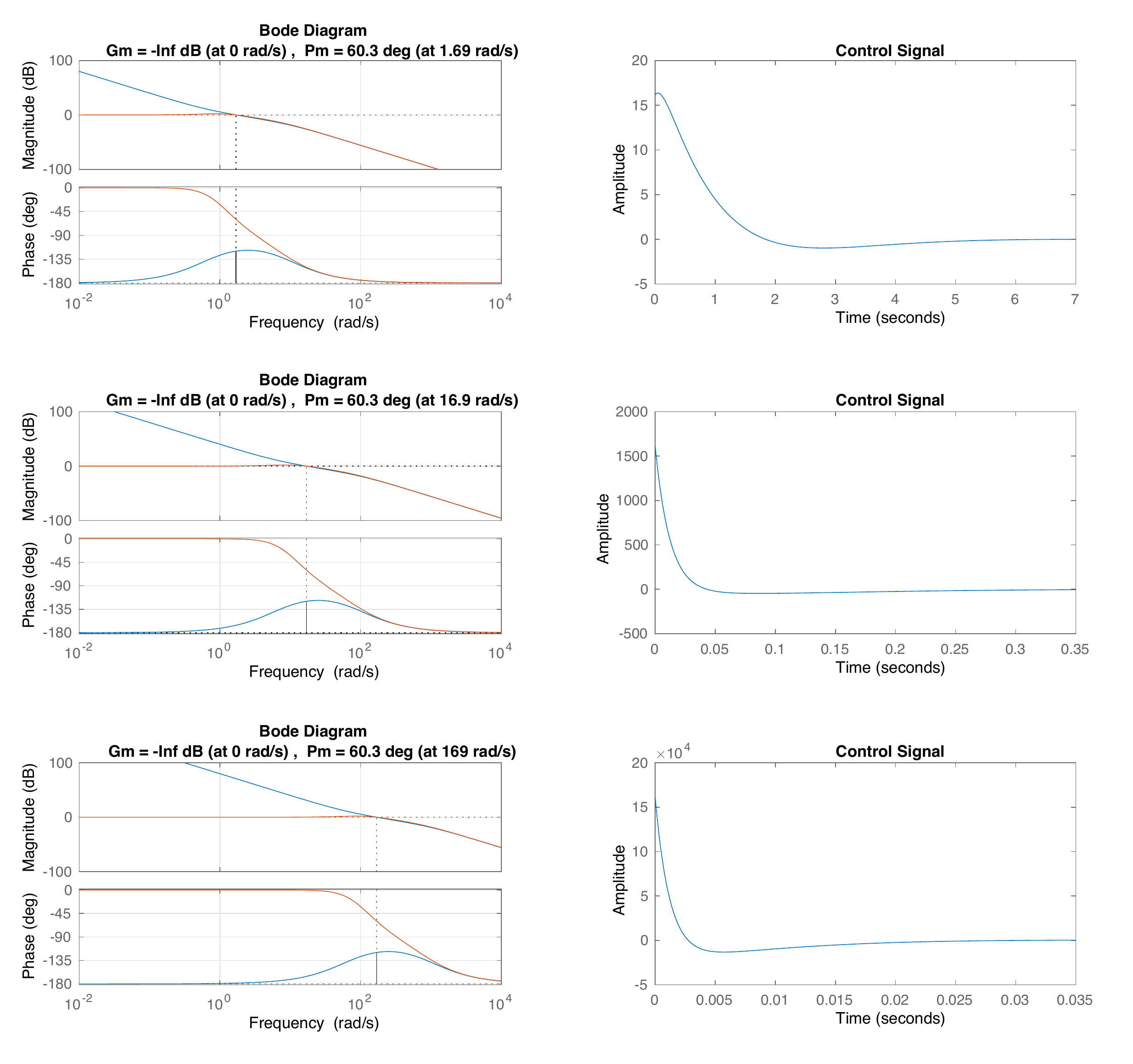
For a given reference signal, the size of the control signal \(u(t)\) is determined by the crossover
frequency. A large crossover frequency will result in a larger control
signal \(u(t)\).
Fig.17.8 shows the open and
closed-loop transfer functions for a plant equal to \(P(s) = \frac{1}{s(s+1)}\) and for three
different controllers that are tuned for equivalent phase margins but
with crossover frequency at \(2\),
\(20\), and \(200\) respectively. The corresponding
control signal when the reference is a unit step is also shown in
Fig.17.8. Note that as \(\omega_{co}\) increases, the magnitude of
the control signal increases and the speed of the response also
increases. In fact, the integral of the control signals will be the same
for each \(\omega_{co}\). Therefore,
saturation constraints on \(u(t)\) will
necessarily limit the size of the crossover frequency \(\omega_{co}\).
Figure 17.8. Closed-loop Bode plot superimposed on the
open-loop Bode plot, together with the corresponding control signal, for
different crossover frequencies.
Chapter 17 interactive figure
Crossover frequency and control effort
Move the
crossover frequency while holding a similar phase-margin trend. The
response gets faster as ωco increases,
but the required control signal grows.
Figure 1.11. Interactive Figure
17.I4. Larger crossover frequency makes the response faster, but
actuator effort increases.
Settling-time
proxy
Peak control
effort
Design warning
17.1.3 Bode Phase Gain
Relationship
In Bode’s original work, he proved the following theorem that relates
the slope of the magnitude plot to the phase.
. For any stable, minimum phase (i.e., zeros in the LHP), linear
time-invariant system \(G(s)\), the
phase of \(G(j\omega)\) is uniquely
related to \(20\log_{10}\left|G(j\omega)\right|\) by
\[\tag{17.1}
\angle G(j\omega_0) = \frac{1}{\pi}\int_{-\infty}^{\infty}
\left(\frac{dM}{du}\right)W(u)\,du,\] where \[\begin{aligned}
M &= 20\log_{10}\left|G(j\omega)\right|, \\
u &= \log_{10}\left|\frac{\omega}{\omega_0}\right|, \\
W(u) &= \log_{10}\left(\coth \frac{\left|u\right|}{2}\right).
\end{aligned}\]
The term \(\frac{dM}{du}\) in
Equation 17.1
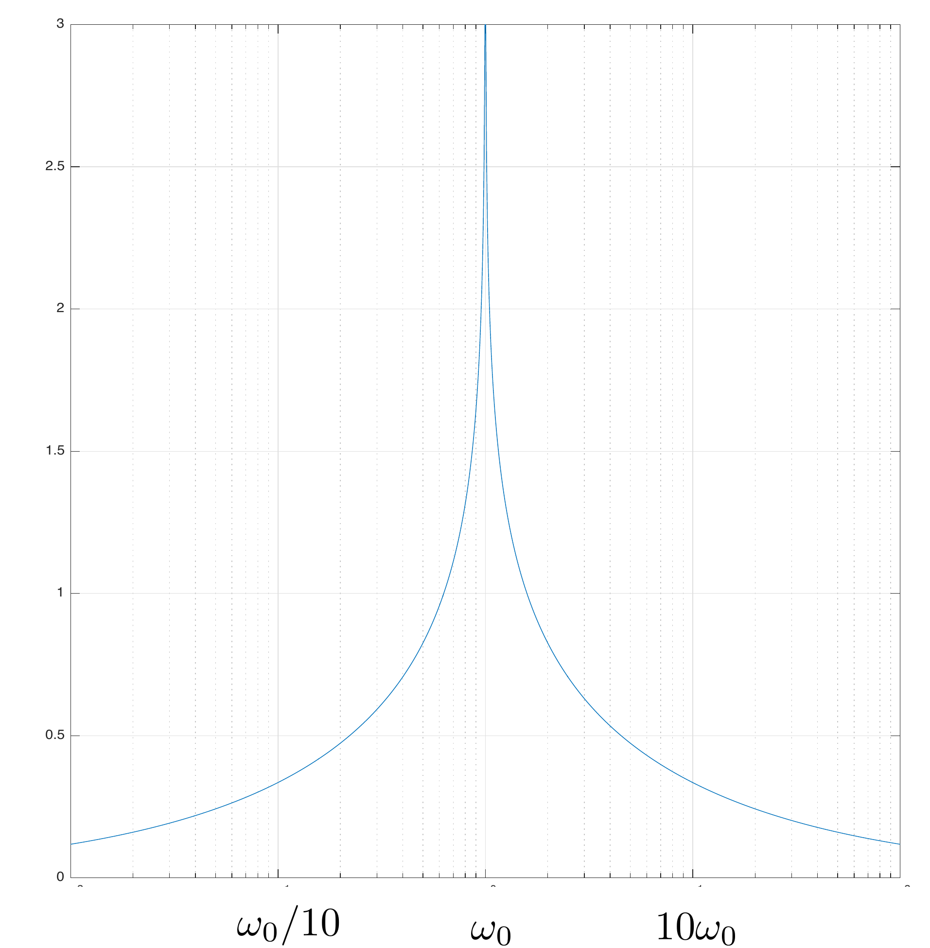
is the slope of the magnitude of \(G(j\omega)\) on the Bode plot. A plot of
\(W(u)\) is shown in
Fig.17.9, where it can be seen that \(W(u)\) heavily weights the slope of the
Bode magnitude around \(\omega_0\), but
also includes bleed-over from the slope for roughly a decade before and
after \(\omega_0\). This implies that
the phase of \(P(j\omega)C(j\omega)\)
at \(\omega=\omega_0\) is determined by
the slope of the Bode magnitude plot in a region about \(\omega_0\).
Figure 17.9. The weighting function W(u) in the Bode gain-phase
relationship heavily weights the slope around ω0.
Recall that the phase for an integrator \(1/s\) is \(-90\) degrees and that the phase for a
differentiator is \(90\) degrees. Also,
recall that the phase for a constant is \(0\) degrees. Therefore, we can approximate
Equation 17.1
as follows:
Of course, these values are approximate and require that the slope
around \(\omega_0\) persist for
approximately a decade before and after \(\omega_0\).
While we do not directly use
Equation 17.1
in practice, it has clear implications for feedback design. In
particular, the takeaway message is that to have a good phase margin,
the slope of the Bode magnitude plot at the crossover frequency \(\omega_{co}\) cannot be too steep, and that
it needs to be reasonably shallow for roughly a decade before and after
crossover. As a rule of thumb, a phase margin of \(PM=60\) degrees requires that the slope at
crossover is between \(-20\) dB/dec and
\(-40\) dB/dec. In other words, the
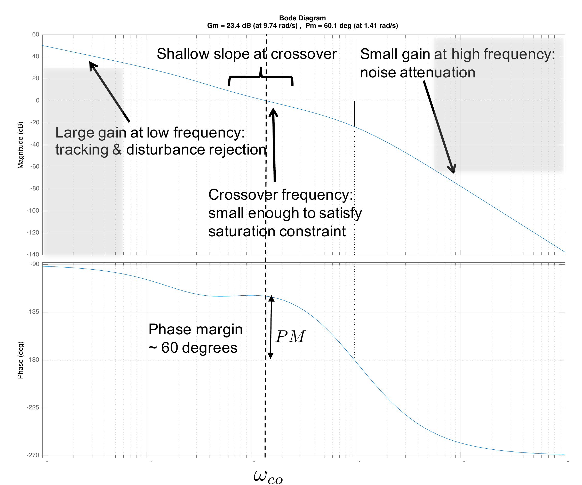
ideal loop shape will need to look something like
Fig.17.10. It is also important to
understand that the Bode phase-gain theorem requires that there is
adequate frequency separation between the frequency content of signals
that we are tracking or rejecting and the frequency content of the
sensor noise that is to be attenuated.
Figure 17.10. The ideal loop shape is large at low
frequencies to achieve good tracking and disturbance rejection, is small
at high frequencies to attenuate sensor noise, has a shallow slope at
the crossover frequency to achieve a good phase margin, and has a small
enough crossover frequency to satisfy the input saturation
constraints.
Chapter 17 interactive figure
Ideal loop-shape checklist
Adjust the loop-shape
parameters and use the checklist to connect the ideal Bode picture in
Figure 17.10 to the design requirement it represents.
Figure 1.12. Interactive Figure 17.I5. Adjust the loop shape
and select checklist items to explain the ideal requirements in
Figure 17.10.
Low-frequency
gainDesign goal:
make the loop gain large at low frequency.
Why it mattersLarge low-frequency loop gain makes
the sensitivity function small where commands and disturbances usually
have most of their energy.
How to check or fix
itCheck that
|PC| is well above 0 dB at low frequency. Increase low-frequency gain
with integral action or lag, but watch the crossover
frequency.
Current checklist
status
Self-checkWhich design action best
supports this region?
For the single-link robot arm, use the bode and
margin commands (from Python or MATLAB) to find the phase
and gain margin for the closed-loop system under PID control. On the
same graph, plot the open-loop Bode plot and the closed-loop Bode plot.
What is the bandwidth of the closed-loop system, and how does this
relate to the crossover frequency? Use the gains found in
HW 3.1.13.
Design Study A guided exercise
Measure stability margins
Use the open-loop Bode plot
to identify crossover, gain margin, phase margin, and bandwidth.
Use this plot to identify gain crossover,
phase margin, gain margin, and closed-loop bandwidth.
Step 1. Gain crossover definition
Show solution for Step
1
Answer: Gain crossover occurs
where the open-loop magnitude is \(0\) dB, or magnitude \(1\).
Step 2. Phase margin reference
Show solution for
Step 2
Answer: Phase margin is the
additional lag needed to reach \(-180^\circ\) at gain crossover.
Step
3. Bandwidth relationship
Show solution for Step
3
Answer: Closed-loop bandwidth is
usually near the open-loop crossover and can be slightly larger for this
design.
Pseudocode
The complete solution includes margin-plot
code. Before opening it, outline how you would compute the open-loop and
closed-loop transfer functions, measure margins, and annotate the Bode
plot.
This prompt is ungraded. It is intended to
connect the margin measurements to the implementation code in the
complete solution.
Complete solution
Python code to generate the plots from this problem is included
below. However, similar MATLAB code is available on the book website
(see http://controlbook.byu.edu).
# 3rd-Partyimport control as cntimport matplotlib.pyplot as plt# local (controlbook)import case_studies.A_arm.params as Pfrom case_studies.A_arm.pid_controller import ArmControllerPIDuse_dB =Falseplant = cnt.tf(P.tf_num, P.tf_den)pid = ArmControllerPID()kp, ki, kd, sigma = pid.kp, pid.ki, pid.kd, pid.sigmacontroller = cnt.tf([kd + kp * sigma, kp + ki * sigma, ki], [sigma, 1, 0])# open-loop systemsys_ol = cnt.series(controller, plant)# closed-loop systemsys_cl = cnt.feedback(sys_ol, 1)if__name__=="__main__":# You could call bode() once with multiple systems, but it draws margins# for all of them. Here we only draw them for the open-loop system.# Calling bode() multiple times reuses the same axes, but removes the title# and legends, so we manually create the figures and axes to add them later. fig, ax = plt.subplots(2, sharex=True) cnt.bode(sys_ol, ax=ax, dB=use_dB, display_margins=True, label="open-loop") cnt.bode(sys_cl, ax=ax, dB=use_dB, grid=False, label="closed-loop")# cross-over frequency ≈ closed-loop bandwidth bandwidth_cl = cnt.bandwidth(sys_cl)print(f"Closed-loop bandwidth: {bandwidth_cl:.2f} rad/s")# Margin info is on the plot, so we don't really need to do this, but this# is how you can calculate it without plotting. gm, pm, wcg, wcp = cnt.margin(sys_ol)print(f"Crossover frequency: {wcp:.2f} rad/s")# draw bandwidth line ax[0].axvline(x=bandwidth_cl, color="red", linestyle=":", label="bandwidth")# manually add annotations after running bode() multiple times ax[0].legend() fig.suptitle("HW 17 Bode Plots: Robot Arm") fig.tight_layout()# keep figure open until closed by user plt.show()
The transfer function for the plant is defined in Line 14. The
transfer function for the PID controller is \[\begin{aligned}
C_{PID}(s) &= k_P + \frac{k_I}{s} + \frac{k_D s}{\sigma s + 1}
= \frac{s(\sigma s+1)k_P + (\sigma s + 1)k_I + k_D
s^2}{s(\sigma s + 1)} \\
&= \frac{(k_D+\sigma k_P)s^2 + (k_P+\sigma k_I)s +
k_I}{s(\sigma s + 1)},
\end{aligned}\] and is defined in Line 15. In Python the
margin command returns information about the phase margin,
gain margin, and frequencies where those are calculated (like the
crossover frequency). The bode command can be used to make
plots of transfer functions (and will show the margin information if
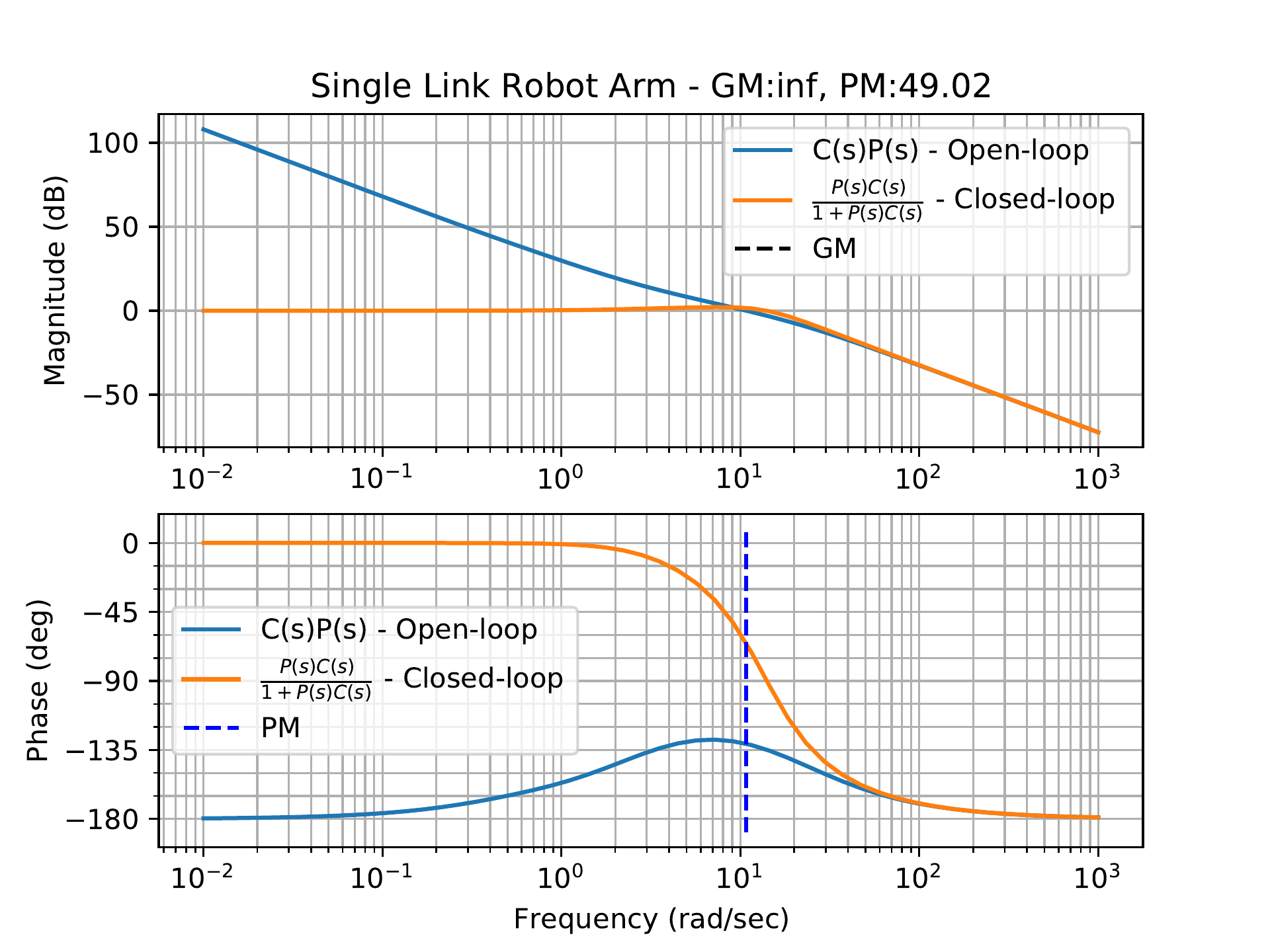
sent the “margin=True” argument). The result of the Python code is shown
in Fig.17.11.
Figure 17.11. Bode plots of the open loop and
closed-loop system for the single-link robot arm under PID
control.
As seen in Fig.17.11
the bandwidth for PID control is approximately \(18\) rad/sec, which is slightly larger than
the crossover frequency of \(10.8\) rad/sec. The larger bandwidth is due
to the small phase margin of \(PM=49.0\) degrees.
For this problem, use the gains found in
HW 3.2.13.
For the inner loop of the inverted pendulum, use the Python or
MATLAB bode and margin commands to find the
phase and gain margin for the inner loop system under PD control. On the
same graph, plot the open-loop Bode plot and the closed-loop Bode plot.
What is the bandwidth of the inner loop, and how does this relate to the
crossover frequency?
For the outer loop of the inverted pendulum, use the
bode and margin commands to find the phase and
gain margin for the outer loop system under PID control. Plot the open
and closed-loop Bode plots for the outer loop on the same plot as the
open and closed-loop Bode plots for the inner loop. What is the
bandwidth of the outer loop, and how does this relate to the crossover
frequency?
What is the bandwidth separation between the inner (fast) loop,
and the outer (slow) loop? For this design, is successive loop closure
justified?
Design
Study B guided exercise
Measure pendulum stability
margins
Compare inner-loop and outer-loop margins and
bandwidths.
Use margin plots to compare crossover, phase
margin, gain margin, and bandwidth.
Step 1.
Inner-loop bandwidth
Show
solution for Step 1
Answer: The
inner-loop bandwidth is approximately 19 rad/s.
Step 2.
Outer-loop bandwidth
Show
solution for Step 2
Answer: The
outer-loop bandwidth is approximately 1.3 rad/s.
Step 3. Bandwidth separation
Show solution for Step
3
Answer: The bandwidths are
separated by about a decade, justifying successive loop
closure.
Pseudocode
The complete solution computes separate
inner-loop and outer-loop margin plots. Before opening it, outline each
component separately.
These prompts are ungraded. They are
intended to connect the derivation to the implementation code in the
complete solution.
Complete solution
second-order The Python code that can be used to generate the plots
for this solution is shown below.
# 3rd-partyimport control as cntimport matplotlib.pyplot as plt# local (controlbook)import case_studies.B_pendulum.params as Pfrom case_studies.B_pendulum.pid_controller import CartPendulumControllerPIDuse_dB =Trueplant_inner = cnt.tf(P.tf_inner_num, P.tf_inner_den)plant_outer = cnt.tf(P.tf_outer_num, P.tf_outer_den)pid = CartPendulumControllerPID()kp_theta, kd_theta, sigma = pid.kp_theta, pid.kd_theta, pid.sigmacontroller_inner = cnt.tf([kd_theta + kp_theta * sigma, kp_theta], [sigma, 1])kp_z, ki_z, kd_z = pid.kp_z, pid.ki_z, pid.kd_zcontroller_outer = cnt.tf( [kd_z + kp_z * sigma, kp_z + ki_z * sigma, ki_z], [sigma, 1, 0])# open-loop systemsys_inner_ol = cnt.series(controller_inner, plant_inner)sys_outer_ol = cnt.series(controller_outer, plant_outer)# closed-loop systemsys_inner_cl = cnt.feedback(sys_inner_ol, 1)sys_outer_cl = cnt.feedback(sys_outer_ol, 1)if__name__=="__main__":# part a)# You could call bode() once with multiple systems, but it draws margins# for all of them. Here we only draw them for the open-loop system.# Calling bode() multiple times reuses the same axes, but removes the title# and legends, so we manually create the figures and axes to add them later. fig, ax = plt.subplots(2, sharex=True) cnt.bode(sys_inner_ol, ax=ax, dB=use_dB, display_margins=True, label="open-loop") cnt.bode(sys_inner_cl, ax=ax, dB=use_dB, grid=False, label="closed-loop")# cross-over frequency ≈ closed-loop bandwidth bandwidth_inner_cl = cnt.bandwidth(sys_inner_cl)print(f"\nClosed-loop bandwidth (inner): {bandwidth_inner_cl:.2f} rad/s")# Margin info is on the plot, so we don't really need to do this, but this# is how you can calculate it without plotting. gm, pm, wcg, wcp = cnt.margin(sys_inner_ol)print(f"Crossover frequency (inner): {wcp:.2f} rad/s")# draw bandwidth line ax[0].axvline(x=bandwidth_inner_cl, color="red", linestyle=":", label="bandwidth")# manually add annotations after running bode() multiple times ax[0].legend() fig.suptitle("HW 17 Bode Plots: Pendulum on a Cart - Inner Loop") fig.tight_layout()# keep figure open until closed by user plt.show()# part b) fig, ax = plt.subplots(2, sharex=True) cnt.bode(sys_outer_ol, ax=ax, dB=use_dB, display_margins=True, label="open-loop") cnt.bode(sys_outer_cl, ax=ax, dB=use_dB, grid=False, label="closed-loop") bandwidth_outer_cl = cnt.bandwidth(sys_outer_cl)print(f"\nClosed-loop bandwidth (outer): {bandwidth_outer_cl:.2f} rad/s") gm, pm, wcg, wcp = cnt.margin(sys_outer_ol)print(f"Crossover frequency (outer): {wcp:.2f} rad/s") ax[0].axvline(x=bandwidth_outer_cl, color="red", linestyle=":", label="bandwidth") ax[0].legend() fig.suptitle("HW 17 Bode Plots: Pendulum on a Cart - Outer Loop") fig.tight_layout() plt.show()# part c) bandwidth_separation = bandwidth_inner_cl / bandwidth_outer_clprint(f"\n{bandwidth_separation =:.2f}")
The transfer functions for the inner and outer loop plants and
controller are defined in Lines 14–19. For this problem, we first
calculate the gain and phase margins (see Lines 26–35). We do this so
that we can then plot the open-loop and closed-loop Bode plots with
stability margin information shown on the plots (see Lines 38–56). If
all we want is the open-loop Bode plot with stability margins, we can
simply pass the argument “margins=True” to the bode
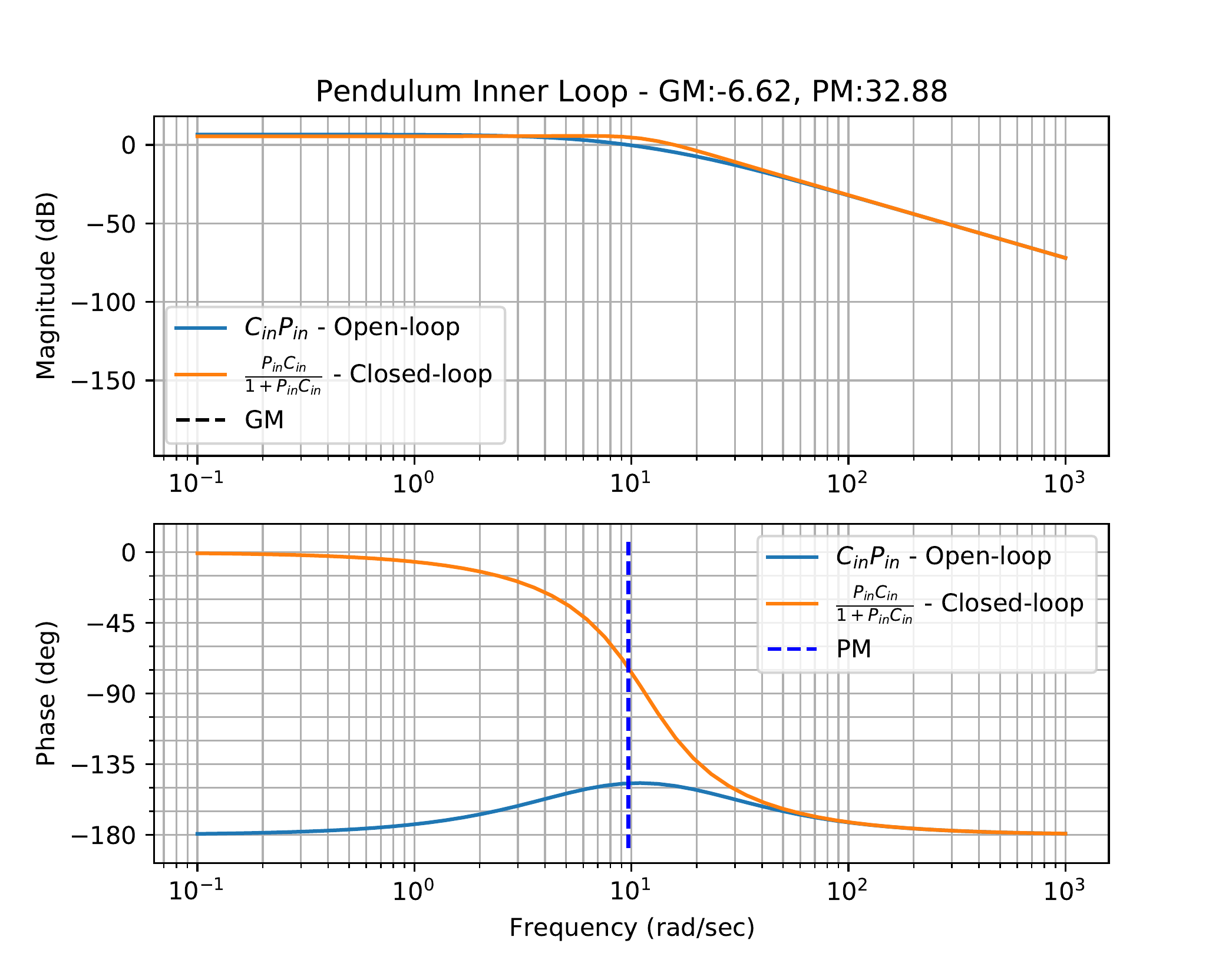
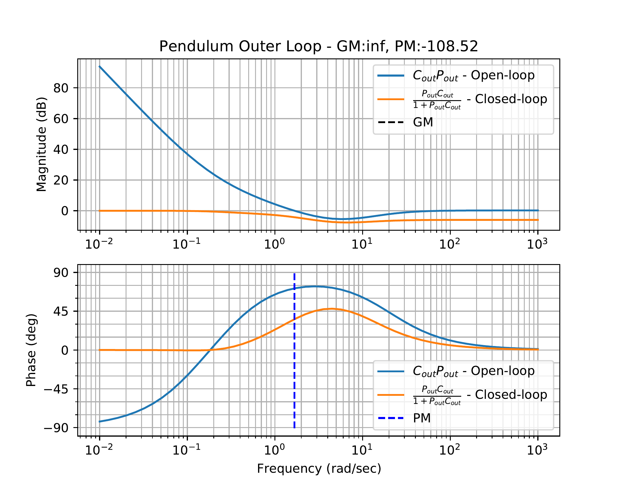
function. The results of this code are shown in Fig.17.12. We follow a
similar process for the outer loop with results shown in
Fig.17.13.
Figure 17.12. Bode plots with stability margins for the
open and closed-loop systems of the inner loop of the inverted pendulum
system.Figure 17.13. Bode plots with stability margins for the
open and closed-loop systems of the outer loop of the inverted pendulum
system.
As seen from Fig.17.12, the bandwidth
of the inner loop is approximately \(19\) rad/sec, which is slightly larger than
the crossover frequency of \(10\) rad/sec. Similarly,
Fig.17.13 indicates that
the bandwidth of the outer loop is approximately \(1.3\) rad/sec, which is slightly larger
than the crossover frequency of \(1.0\) rad/sec with a phase margin of \(PM=72\) degrees (the plot says -108, but
this is off by \(180\), so that \(PM = 180-108\)).
For a second-order system, making the step response 10 times faster
implies that \(t_r\) is divided by 10,
or equivalently that \(\omega_n\) is
multiplied by 10. A similar principle holds for high order systems. To
be 10 times faster, the closed-loop bandwidth of the inner loop should
be a decade higher on the Bode plot than the closed-loop bandwidth of
the outer loop. The bandwidth separation between the inner and outer
loop is about one decade justifying the successive loop closure design
approach.
For this problem, use the gains found in
HW 3.3.13.
For the inner loop of the satellite attitude controller, use the
bode and margin commands (from MATLAB or
Python) to find the phase and gain margin for the inner loop system
under PD control. On the same graph, plot the open-loop Bode plot and
the closed-loop Bode plot. What is the bandwidth of the closed-loop
system, and how does this relate to the crossover frequency?
For the outer loop of the satellite attitude controller, use the
bode and margin commands to find the phase and
gain margin for the outer loop system under PID control. Plot the open
and closed-loop Bode plots for the outer loop on the same plot as the
open and closed-loop Bode plots for the inner loop. What is the
bandwidth of the closed-loop system, and how does this relate to the
crossover frequency?
What is the bandwidth separation between the inner (fast) loop,
and the outer (slow) loop? For this design, is successive loop closure
justified?
Design Study C guided exercise
Measure satellite stability margins
Compare the inner
and outer loop crossover frequencies, phase margins, bandwidths, and
bandwidth separation.
Step 1. Inner-loop margin context
Show
solution for Step 1
Answer: The
inner-loop bandwidth is about 11 rad/s with phase margin about 56
degrees.
Step 2. Outer-loop margin context
Show
solution for Step 2
Answer: The
outer-loop bandwidth is about 1 rad/s, giving close to a decade of
separation.
Step 3.
Successive-loop closure judgment
Show solution for Step
3
Answer: Yes, the bandwidths are
close to a decade apart and the closed inner loop is approximately one
over the outer-loop bandwidth.
Complete solution
Python code to generate the plots in this solution is included
below.
# 3rd-partyimport control as cntimport matplotlib.pyplot as plt# local (controlbook)import case_studies.C_satellite.params as Pfrom case_studies.C_satellite.pid_controller import SatelliteControllerPIDuse_dB =Trueplant_inner = cnt.tf(P.tf_inner_num, P.tf_inner_den)plant_outer = cnt.tf(P.tf_outer_num, P.tf_outer_den)pid = SatelliteControllerPID()kp_theta, kd_theta, sigma = pid.kp_theta, pid.kd_theta, pid.sigmacontroller_inner = cnt.tf([kd_theta + kp_theta * sigma, kp_theta], [sigma, 1])kp_phi, ki_phi, kd_phi = pid.kp_phi, pid.ki_phi, pid.kd_phicontroller_outer = cnt.tf( [kd_phi + kp_phi * sigma, kp_phi + ki_phi * sigma, ki_phi], [sigma, 1, 0])# open-loop systemsys_inner_ol = cnt.series(controller_inner, plant_inner)sys_outer_ol = cnt.series(controller_outer, plant_outer)# closed-loop systemsys_inner_cl = cnt.feedback(sys_inner_ol, 1)sys_outer_cl = cnt.feedback(sys_outer_ol, 1)if__name__=="__main__":# part a)# You could call bode() once with multiple systems, but it draws margins# for all of them. Here we only draw them for the open-loop system.# Calling bode() multiple times reuses the same axes, but removes the title# and legends, so we manually create the figures and axes to add them later. fig, ax = plt.subplots(2, sharex=True) cnt.bode(sys_inner_ol, ax=ax, dB=use_dB, display_margins=True, label="open-loop") cnt.bode(sys_inner_cl, ax=ax, dB=use_dB, grid=False, label="closed-loop")# cross-over frequency ≈ closed-loop bandwidth bandwidth_inner_cl = cnt.bandwidth(sys_inner_cl)print(f"\nClosed-loop bandwidth (inner): {bandwidth_inner_cl:.2f} rad/s")# Margin info is on the plot, so we don't really need to do this, but this# is how you can calculate it without plotting. gm, pm, wcg, wcp = cnt.margin(sys_inner_ol)print(f"Crossover frequency (inner): {wcp:.2f} rad/s")# draw bandwidth line ax[0].axvline(x=bandwidth_inner_cl, color="red", linestyle=":", label="bandwidth")# manually add annotations after running bode() multiple times ax[0].legend() fig.suptitle("HW 17 Bode Plots: Satellite - Inner Loop") fig.tight_layout()# keep figure open until closed by user plt.show()# part b) fig, ax = plt.subplots(2, sharex=True) cnt.bode(sys_outer_ol, ax=ax, dB=use_dB, display_margins=True, label="open-loop") cnt.bode(sys_outer_cl, ax=ax, dB=use_dB, grid=False, label="closed-loop") bandwidth_outer_cl = cnt.bandwidth(sys_outer_cl)print(f"\nClosed-loop bandwidth (outer): {bandwidth_outer_cl:.2f} rad/s") gm, pm, wcg, wcp = cnt.margin(sys_outer_ol)print(f"Crossover frequency (outer): {wcp:.2f} rad/s") ax[0].axvline(x=bandwidth_outer_cl, color="red", linestyle=":", label="bandwidth") ax[0].legend() fig.suptitle("HW 17 Bode Plots: Satellite - Outer Loop") fig.tight_layout() plt.show()# part c) bandwidth_separation = bandwidth_inner_cl / bandwidth_outer_clprint(f"\n{bandwidth_separation =:.2f}")
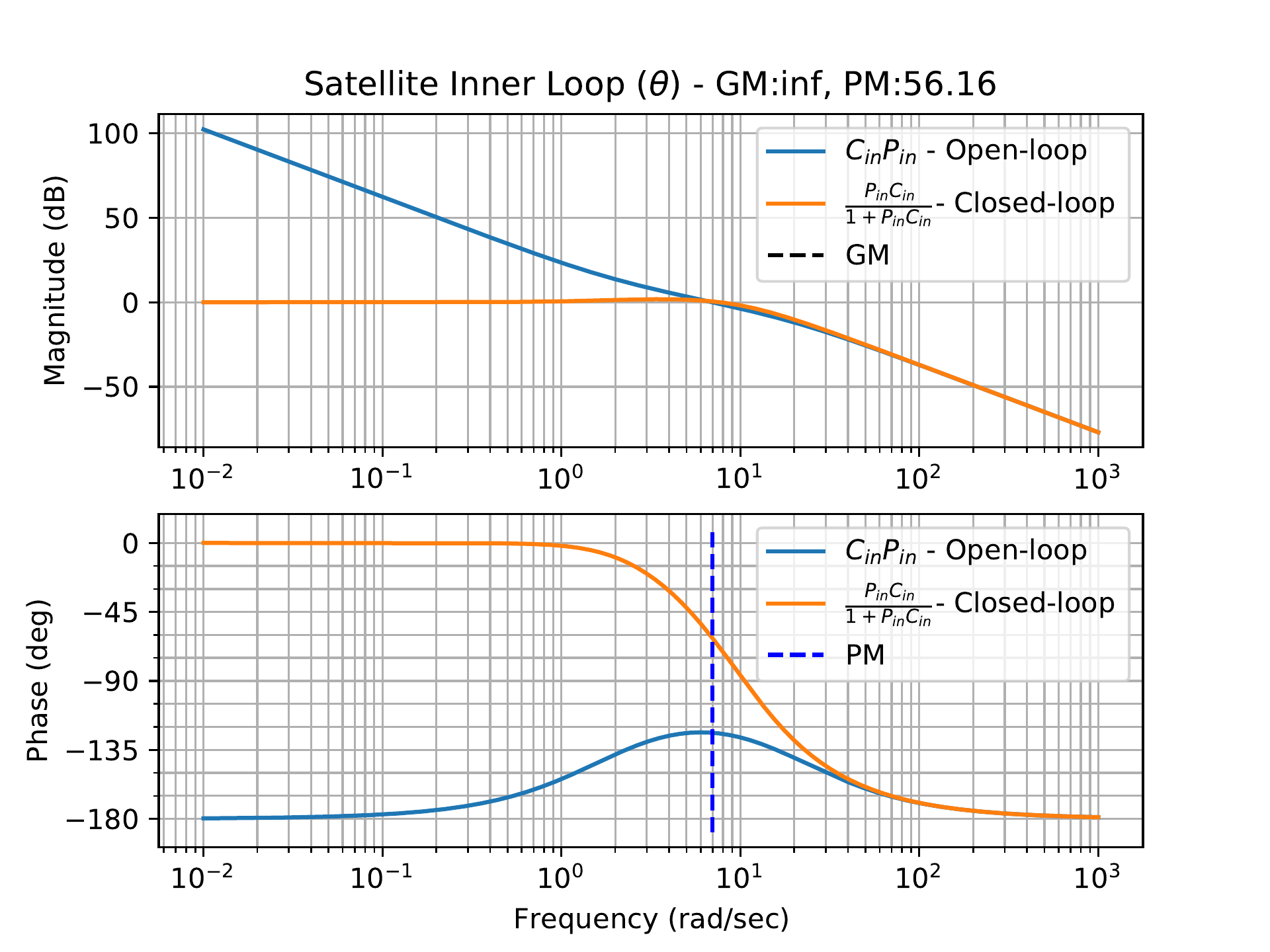
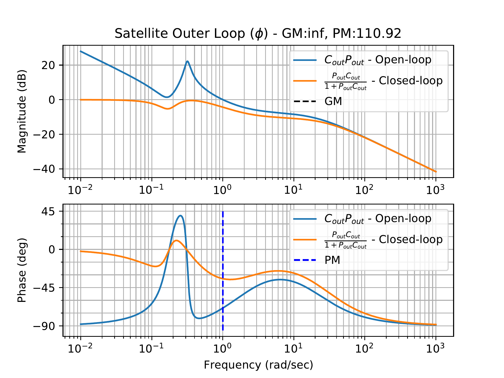
Similar to the last two case studies, the transfer functions for the
inner and outer loop plants are calculated first. Then we find the
stability margins and generate Bode plots for the inner loop (see
Fig.17.14). We follow
the same procedure for the outer loop plots shown in
Fig.17.15.
Figure 17.14. Bode plots with stability margins for the
open and closed-loop systems of the inner loop of the satellite
system.Figure 17.15. Bode plots with stability margins for the
open and closed-loop systems of the outer loop of the satellite
system.
As shown in Fig.17.14, the bandwidth
of the inner loop is approximately \(11\) rad/sec, which is slightly larger than
the crossover frequency of \(7\) rad/sec, with a phase margin of \(PM=56\) degrees. Similarly,
Fig.17.15 indicates that
the bandwidth of the outer loop is approximately the crossover frequency
of \(1\) rad/sec. The bandwidth
separation between the inner and outer loops is close to a decade, and
the magnitude of the inner-loop closed-loop frequency response is
approximately one at frequencies well above the crossover frequency of
the outer loop.
17.5 Coding Lab: Stability
Margins
Objective: estimate gain crossover, phase
margin, phase crossover, and gain margin from sampled Bode data.
Evaluation criteria: the lab checks
interpolation at crossover points and compares the computed margins to a
reference result.
Figure 17.1 (Interactive). Stability-margin coding lab with crossover
annotations.
17.6 Knowledge Check
Q1. Phase margin
location
Phase margin is measured
at:
Q2.
Gain margin location
Gain margin is
measured relative to:
Q3. Phase margin calculation
If the phase at gain crossover is -135 degrees, enter the phase margin
in degrees.
Show solution
Answer: 45 degrees because the phase is 45 degrees
above -180 degrees.
Q4. Gain margin calculation
At phase crossover, the magnitude is -8 dB. Enter the gain margin in dB.
Show solution
Answer: 8 dB because the gain could increase by 8 dB
before reaching 0 dB at phase crossover.
Q5. Missing crossover
If the Bode plot has no gain crossover, what should you say about phase
margin?
Show solution
Answer: It is undefined or does not exist because there
is no gain-crossover frequency where it can be measured.
Q6. Phase margin
readout
At the gain-crossover
frequency, the phase is -140 degrees. What is the phase margin?
Q7. Gain margin readout
At phase
crossover, the magnitude is -12 dB. What is the gain margin?
Q8. Gain increase consequence
What commonly happens when loop gain is increased
in a system whose phase becomes more negative at higher frequency?
Q9.
Missing phase crossover
If the Bode
plot does not show a phase crossover in the plotted frequency range,
what should you conclude about gain margin from that plot alone?