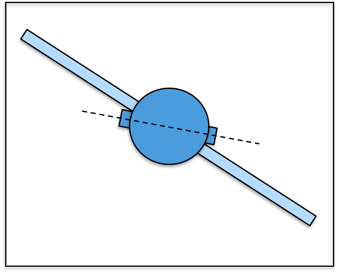
In Part III we focused on designing feedback control systems for second-order systems. Since second-order systems have two poles, we saw that it is possible to use feedback control with two gains to place the closed-loop poles at any desired location. In Chapter 14 of this book we will see that for an \(n^{th}\) order system it is possible to arbitrarily place the closed-loop poles, but that this will require \(n\) feedback gains. In that sense, the full state feedback controllers that we will derive in Chapter 14 are a generalization of PD control to higher-order systems. This generalization is most easily accomplished using the state-space model of the system derived in Chapter 9. In fact, the state-space model leads to efficient numerical routines for designing and implementing the feedback controller.

In Chapter 15 we show how integral control can be added to the state feedback controllers designed in Chapter 14. The method introduced in Chapter 15 has a significant advantage over the integrator tuning method discussed in Chapter 13 in the sense that tuning the integral gain will not impact the other closed-loop poles and therefore allows for greater design flexibility.

We saw in Chapter 13 that in order to implement PD/PID control, the derivative of the output needs to be reconstructed using a digital differentiator. The generalization of this idea to state feedback control is that the full state of the system must be reconstructed. The tool that we will use to reconstruct the system state is called an observer. The observer design problem will be discussed in Chapter 16.

It turns out that observers can be used in a variety of different contexts outside of feedback control. In particular, observers can be used to solve target tracking problems and to estimate the system parameters of complex dynamic systems. In the setting of feedback control where unknown input and output disturbances act on the system, observers can be used to estimate the unknown disturbances. In Chapter 17 we will show how to design the observer to estimate both the system state and the unknown constant input disturbance. We will also show that estimating the input disturbance is mathematically and functionally similar to adding an integrator.

The design tools developed in Part IV of this book use state-space models and require the use of linear algebra and matrix analysis. A brief review of linear algebra concepts that will be used in Part IV are given in Appendix 31.

11 Full State Feedback

11.1 Theory

In this chapter we will show how to use full state feedback to stabilize a linear time-invariant system represented in state-space form. Recall from Section 9.1.2, that for state-space equations given by \begin{align} \dot{x} &= Ax + Bu \tag{11.1}\\ y &= Cx + Du, \tag{11.2} \end{align} the poles of the system are the eigenvalues of \(A\), or in other words, the roots of the open-loop characteristic equation \[\Delta_{ol}(s) = \det(sI-A) = 0.\] The matrix \(A\) is called the state-interaction matrix because it specifies how the states interact with each other. The basic idea behind full state feedback is to use the feedback signal to change the interaction matrix so that the poles are in specified locations. A full state feedback controller is given by \[\tag{11.3} u = -Kx + \nu,\] where \(K\in\mathbb{R}^{m\times n}\) are the feedback gains, and \(\nu\) will be a signal that is specified later. Using 11.3 in Equation 11.1 results in the closed-loop state-space equations \begin{align} \dot{x} &= Ax + B(-Kx+\nu) = (A-BK)x + B\nu \tag{11.4}\\ y &= Cx, \tag{11.5} \end{align} where the interaction matrix is now \(A-BK\), and so the closed-loop poles will be given by the eigenvalues of \(A-BK\), or in other words, the roots of the closed-loop characteristic equation \[\Delta_{cl}(s) = \det(sI-(A-BK))=0.\] A natural question that will be addressed in the remainder of this section is how to select \(K\) so that the closed-loop characteristic equation is equal to a desired closed-loop characteristic polynomial \(\Delta_{cl}^d(s)\), where the designer selects the roots of \(\Delta_{cl}^d(s)=0\) to achieve the desired closed-loop performance.

Section 9.1.2 showed that the state-space model given by Equations 11.1–11.2 is equivalent to the transfer function model given by \[\tag{11.6} Y(s) = C(sI-A)^{-1}B U(s).\] While the mapping from state-space model to transfer function model is unique, the reverse is not true. In fact, there are an infinite number of state-space models that correspond to a particular transfer function model. Accordingly, we say that a state-space model is a realization of the transfer function model, if it produces the same input-output behavior when the initial conditions are zero.

In particular, define the change of variables \[\tag{11.7} z = P^{-1}x,\] where \(P\) is an invertible matrix. Then \begin{align} \dot{z} &= P^{-1}\dot{x} = P^{-1}(Ax+Bu) = P^{-1}APz + P^{-1}B u \tag{11.8}\\ y&= Cx = CPz \tag{11.9} \end{align} is an alternative state-space representation of system 11.1-11.2. To show that these two representations have the same input-output behavior, or in other words, the same transfer function, note from Equation 11.6 that the transfer function of system 11.8-11.9 is \[\begin{aligned} Y(s) &= \left( CP(sI-P^{-1}AP)^{-1}P^{-1}B \right) U(s) \\ &= \left( CP(sP^{-1}P-P^{-1}AP)^{-1}P^{-1}B\right) U(s) \\ &= \left( CP(P^{-1}(sI-A)P)^{-1}P^{-1}B \right) U(s) \\ &= \left( CPP^{-1}(sI-A)^{-1}PP^{-1}B \right) U(s) \\ &= \left( C(sI-A)^{-1}B \right) U(s), \end{aligned}\] which is identical to Equation 11.6. Therefore, Equations 11.1-11.2 and Equations 11.8-11.9 are realizations of the same system.

11.1.1 State-Space Realization in Control Canonic Form

In this section, we will derive one specific state-space realization for single-input single-output transfer functions, where the state feedback problem is particularly simple. The realization that we derive below is called the control canonic form of the system.

Consider the general SISO monic transfer function model given by \[\tag{11.10} Y(s) = \frac{b_ms^m + b_{m-1}s^{m-1} + \dots + b_1 s + b_0}{s^n + a_{n-1}s^{n-1} + \dots + a_1 s + a_0} U(s),\] where \(m<n\). The block diagram of the system is shown in Fig. 11.1.

The first step in deriving the control canonic state-space equations is to artificially decompose the transfer function as shown in Fig. 11.2, where the numerator polynomial and the denominator polynomial appear in separate cascaded blocks, and where \(Z(s)\) is an artificial intermediate variable.

In the \(s\)-domain, the equations corresponding to Fig. 11.2 can be written as \[\begin{aligned} Z(s) &= \frac{1}{s^n + a_{n-1}s^{n-1} + \dots + a_1 s + a_0} U(s) \\ Y(s) &= (b_ms^m + b_{m-1}s^{m-1} + \dots + b_1 s + b_0) Z(s). \end{aligned}\] Taking the inverse Laplace transform of these equations gives \begin{align} \frac{d^nz}{dt^n} &= u(t) - a_{n-1}\frac{d^{n-1}z}{dt^{n-1}} - \dots - a_1 \dot{z} - a_0 z(t) \tag{11.11}\\ y(t) &= b_m\frac{d^mz}{dt^m} + b_{m-1}\frac{d^{m-1}z}{dt^{m-1}} + \dots + b_1 \dot{z} + b_0 z(t). \tag{11.12} \end{align}

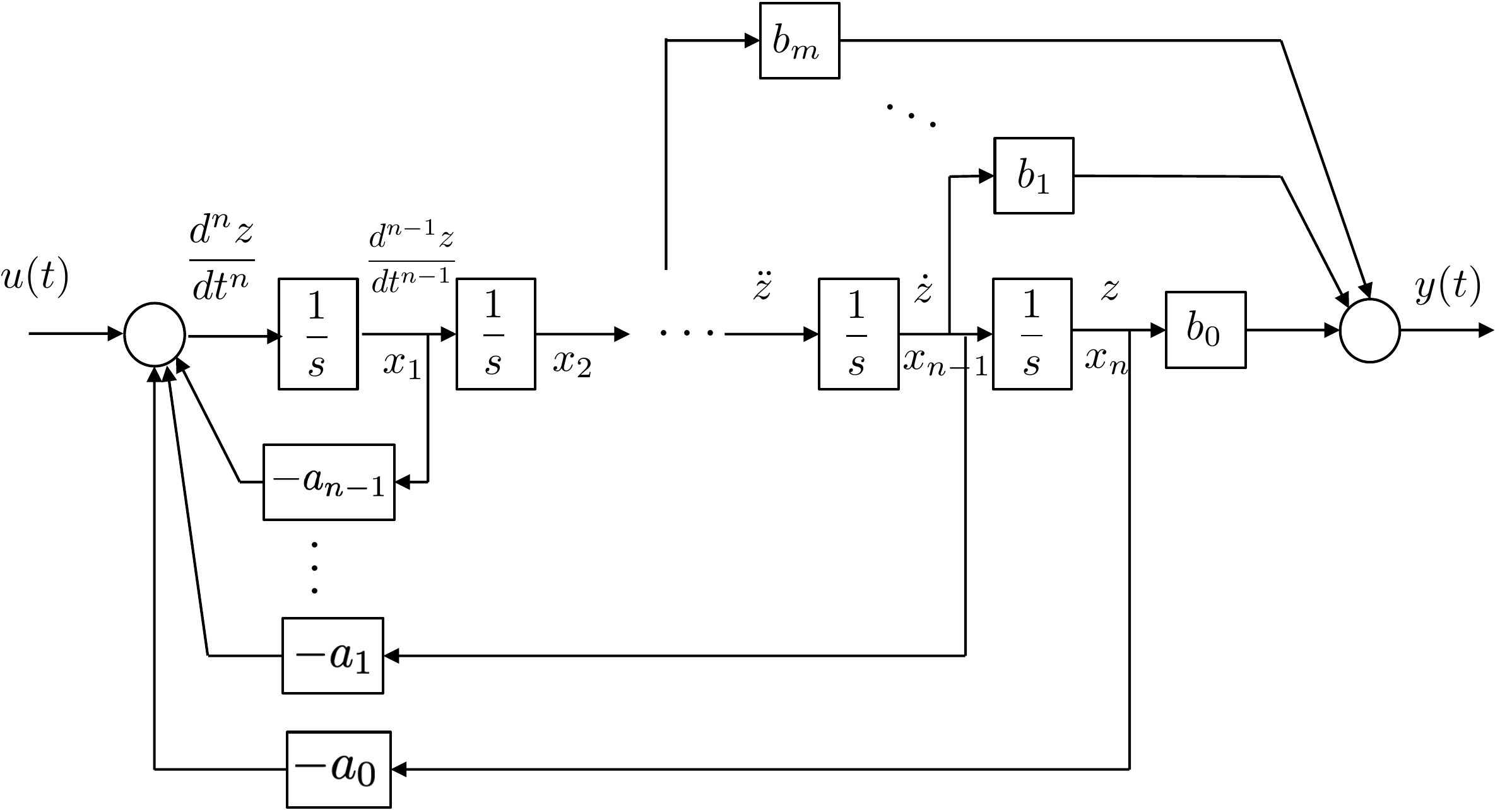
The next step in the derivation of the state-space equations is to draw the analog computer implementation of Equations 11.11 and 11.12, which is shown in Fig. 11.3.

Labeling the output of the integrators as the state variables \(x_1, \dots, x_n\), as shown in Fig. 11.3, we can write the state-space equations as \begin{align} \begin{pmatrix} \dot{x}_1 \\ \dot{x}_2 \\ \vdots \\ \dot{x}_n \end{pmatrix} &= \begin{pmatrix} -a_{n-1} & -a_{n-2} & \dots & -a_1 & -a_0 \\ 1 & 0 & \dots & 0 & 0 \\ 0 & 1 & \dots & 0 & 0 \\ \vdots & & \ddots & & \vdots \\ 0 & 0 & \dots & 1 & 0 \end{pmatrix} \begin{pmatrix} x_1 \\ x_2 \\ \vdots \\ x_n \end{pmatrix} + \begin{pmatrix} 1 \\ 0 \\ \vdots \\ 0 \end{pmatrix} u \tag{11.13} \\ y &= \begin{pmatrix} 0 & \dots & 0 & b_m & \dots & b_1 & b_0 \end{pmatrix} \begin{pmatrix} x_1 \\ x_2 \\ \vdots \\ x_n \end{pmatrix} + 0\cdot u. \notag \end{align} In the case when \(m=n\) it is straightforward to show that the output equation becomes \[y = \begin{pmatrix} b_{n-1} - b_n a_{n-1}, & \dots & b_1 - b_n a_1, & b_0 - b_n a_0 \end{pmatrix} \begin{pmatrix} x_1 \\ x_2 \\ \vdots \\ x_n \end{pmatrix} + b_n\cdot u.\] We will define the control canonic realization as \[\begin{aligned} \dot{x}_c &= A_c x_c + B_c u \\ y &= C_c x_c + Du, \end{aligned}\] where \begin{align} A_c &\stackrel{\triangle}{=}\begin{pmatrix} -a_{n-1} & -a_{n-2} & \dots & -a_1 & -a_0 \\ 1 & 0 & \dots & 0 & 0 \\ 0 & 1 & \dots & 0 & 0 \\ \vdots & & \ddots & & \vdots \\ 0 & 0 & \dots & 1 & 0 \end{pmatrix} \tag{11.14}\\ B_c &\stackrel{\triangle}{=}\begin{pmatrix} 1 \\ 0 \\ \vdots \\ 0 \end{pmatrix} \tag{11.15} \\ C_c &\stackrel{\triangle}{=}\begin{cases} \begin{pmatrix} 0 & \dots & 0 & b_m & \dots & b_1 & b_0 \end{pmatrix} &\quad m<n \\ \begin{pmatrix} b_{n-1} - b_n a_{n-1}, & \dots & b_1 - b_n a_1, & b_0 - b_n a_0 \end{pmatrix} &\quad m=n \end{cases} \tag{11.16} \\ D &\stackrel{\triangle}{=}\begin{cases} 0 &\quad m<n \\ b_n &\quad m=n \end{cases}. \tag{11.17} \end{align} Note that the negative of the coefficients of the denominator of 11.10 constitute the first row of \(A_c\), and that the remainder of \(A_c\) has ones on the lower off diagonal and zeros in all other elements. Matrices with this structure are said to be in companion form. The \(B_c\) vector has a single one as its first element, with the remaining elements equal to zero. The coefficients of the numerator of Equation 11.10 are the last \(p\)-elements of \(C_c\).

As an example, suppose that the transfer function model of the system is given by \[Y(s) = \frac{9s + 20}{s^3 + 6s^2 - 11s + 8}U(s),\] then the control canonic realization of the system is given by \begin{align} \begin{pmatrix} \dot{x}_1 \\ \dot{x}_2 \\ \dot{x}_3 \end{pmatrix} &= \begin{pmatrix} -6 & 11 & -8 \\ 1 & 0 & 0 \\ 0 & 1 & 0 \end{pmatrix}\begin{pmatrix} x_1 \\ x_2 \\ x_3 \end{pmatrix} + \begin{pmatrix} 1 \\ 0 \\ 0\end{pmatrix} u \tag{11.18} \\ y &= \begin{pmatrix} 0 & 9 & 20 \end{pmatrix} \begin{pmatrix} x_1 \\ x_2 \\ x_3 \end{pmatrix}. \notag \end{align}

11.1.2 Full State Feedback using Control Canonic Form

The design of a state feedback controller is particularly easy when the state-space equations are in control canonic form. The key insight is that there is a direct relationship between matrices in companion form, as shown in Equation 11.14 and their characteristic polynomial \[\Delta_{ol}(s) = s^n + a_{n-1}s^{n-1} + \dots + a_1 s + a_0.\] Suppose that we let \[\tag{11.19} u = -K_cx_c + \nu = -\begin{pmatrix} k_1 & k_2 & \dots & k_{n-1} & k_n\end{pmatrix} \begin{pmatrix} x_1 \\ x_2 \\ \vdots \\ x_{n-1} \\ x_n \end{pmatrix} + \nu.\] Substituting into Equation 11.13 and rearranging gives \[\begin{gathered} \begin{pmatrix} \dot{x}_1 \\ \dot{x}_2 \\ \vdots \\ \dot{x}_n \end{pmatrix} = \begin{pmatrix} -(a_{n-1}+k_1) & -(a_{n-2}+k_2) & \dots & -(a_1+k_{n-1}) & -(a_0+k_n) \\ 1 & 0 & \dots & 0 & 0 \\ 0 & 1 & \dots & 0 & 0 \\ \vdots & & \ddots & & \vdots \\ 0 & 0 & \vdots & 1 & 0 \end{pmatrix} \begin{pmatrix} x_1 \\ x_2 \\ \vdots \\ x_n \end{pmatrix} % + \begin{pmatrix} 1 \\ 0 \\ \vdots \\ 0 \end{pmatrix} \nu. \end{gathered}\] Since the state interaction matrix is still in companion form, the characteristic polynomial of the closed-loop system is given by \[\Delta_{cl}(s) = s^n + (a_{n-1}+k_1)s^{n-1} + \dots + (a_1+k_{n-1}) s + (a_0+k_n).\] If the desired characteristic polynomial is given by \[\tag{11.20} \Delta_{cl}^d(s) = s^n + \alpha_{n-1}s^{n-1} + \dots + \alpha_1 s + \alpha_0,\] then we have that \[\begin{aligned} a_{n-1} + k_1 &= \alpha_{n-1} \\ a_{n-2} + k_2 &= \alpha_{n-2} \\ \vdots & \\ a_{1} + k_{n-1} &= \alpha_{1} \\ a_0 + k_n &= \alpha_0. \end{aligned}\] Defining the row vectors \[\begin{aligned} \mathbf{a}_A &= (a_{n-1}, a_{n-2}, \dots, a_1, a_0) \\ \boldsymbol{\alpha} &= (\alpha_{n-1}, \alpha_{n-2}, \dots, \alpha_1, \alpha_0) \\ K_c &= (k_1, k_2, \dots, k_{n-1}, k_n), \end{aligned}\] we have that the feedback gains satisfy \[\tag{11.21} K_c = \boldsymbol{\alpha}-\mathbf{a}_A,\] where the subscript “c” is used to emphasize that the gains are in control canonic form.

As an example, consider the state equations given in Equation 11.18. The open-loop characteristic polynomial is given by \[\Delta_{ol}(s) = s^3 + 6s^2 - 11 s + 8,\] with roots at \(-7.5885\), and \(0.7942\pm j0.6507\). Suppose that the desired closed-loop characteristic polynomial is \[\Delta_{cl}^d(s) = s^3 + 5s^2 + 12 s + 8,\] with roots at \(-1\) and \(-2\pm j2\), then \(\mathbf{a}_A = (6, -11, 8)\), and \(\boldsymbol{\alpha} = (5, 12, 8)\). The feedback gains that place the poles at the desired locations are therefore given by \[K_c = \boldsymbol{\alpha}-\mathbf{a}_A = (5, 12, 8)-(6, -11, 8) = (-1, 23, 0).\]

11.1.3 Full State Feedback: General Case

The formula given in Equation 11.21 assumes that the state-space equations are in control canonic form. It turns out that the closed-loop eigenvalues cannot always be arbitrarily assigned to desired locations. When they can, the system \(\dot{x}=Ax+Bu\) is said to be controllable. In this section we will derive an expression for the state feedback gains, and we will simultaneously derive a simple test for determining when the system is controllable.

Recall from Equations 11.7–11.9 that state-space equations can be transformed using the change of variables in Equation 11.7 without modifying the input-output properties of the system. This implies that the change of variables does not change the characteristic polynomial. We can verify this fact explicitly as follows: \[\begin{aligned} \det(sI-P^{-1}AP) &= \det(sP^{-1}P-P^{-1}AP) \\ &= \det\left(P^{-1}(sI-A)P\right) \\ &= \det(P^{-1})\det(sI-A)\det(P) \\ &= \det(sI-A). \end{aligned}\]

Therefore, to derive full state feedback gains for the general state-space equations \[\tag{11.22} \dot{x}=Ax+Bu,\] the idea is to find a state transformation matrix \(P\) so that the transformed system is in control canonic form, i.e., find \(P\) so that \[\tag{11.23} x_c=P^{-1}x,\] and \[\tag{11.24} \dot{x}_c = P^{-1}APx_c + P^{-1}B u = A_c x_c + B_c u,\] where \(A_c\) and \(B_c\) have the form given by Equations 11.14 and 11.15, respectively. Therefore, we need to find \(P\) so that \(P^{-1}B = B_c\), and \(P^{-1}AP=A_c\), which are satisfied if and only if \(B=PB_c\) and \(AP=PA_c\). Let \(P=(\mathbf{p}_1, \mathbf{p}_2, \dots, \mathbf{p}_n)\), where \(\mathbf{p}_i\in\mathbf{R}^n\) is the \(i^{th}\) column of \(P\). The requirement that \(B=PB_c\) implies that \[B = \begin{pmatrix} \mathbf{p}_1 & \mathbf{p}_2 & \dots & \mathbf{p}_n \end{pmatrix} \begin{pmatrix} 1 \\ 0 \\ \vdots \\ 0 \end{pmatrix} = \mathbf{p}_1.\] Therefore, \(\mathbf{p}_1=B\). The requirement that \(PA_c=AP\) implies that \[\begin{gathered} \begin{pmatrix} \mathbf{p}_1 & \mathbf{p}_2 & \dots & \mathbf{p}_n \end{pmatrix}\begin{pmatrix} -a_{n-1} & -a_{n-2} & \dots & -a_1 & -a_0 \\ 1 & 0 & \dots & 0 & 0 \\ 0 & 1 & \dots & 0 & 0 \\ \vdots & & \ddots & & \vdots \\ 0 & 0 & \dots & 0 & 0 \\ 0 & 0 & \vdots & 1 & 0 \end{pmatrix} \\ = A \begin{pmatrix} \mathbf{p}_1 & \mathbf{p}_2 & \dots & \mathbf{p}_n \end{pmatrix}. \end{gathered}\] After multiplication, the first \(n-1\) columns can be equated to get \begin{align} -a_{n-1}\mathbf{p}_1 + \mathbf{p}_2 &= A\mathbf{p}_1 \tag{11.25}\\ -a_{n-2}\mathbf{p}_1 + \mathbf{p}_3 &= A\mathbf{p}_2 \tag{11.26}\\ \vdots \\ -a_1\mathbf{p}_1 + \mathbf{p}_{n} &= A\mathbf{p}_{n-1}. \tag{11.28} \end{align} Equation 11.25, and the previous conclusion that \(\mathbf{p}_1=B\), implies that \[\mathbf{p}_2 = a_{n-1}B + AB.\] Using this result in Equation 11.26 gives \[\mathbf{p}_3 = a_{n-2}B + a_{n-1} AB + A^2B.\] We can continue to iteratively solve for each column of \(P\) until the \((n-1)^{th}\) column, which from Equation 11.28 is \[\mathbf{p}_n = a_1B + a_2AB + \dots + a_{n-1}A^{n-2}B + A^{n-1}B.\] Notice that each column in \(P\) is a linear combination of the elements \(B\), \(AB\), \(A^2B\), \(\dots\), \(A^{n-1}B\). Accordingly, defining \[\tag{11.29} \mathcal{C}_{A,B} = \begin{pmatrix} B & AB & A^2B & \dots & A^{n-1}B\end{pmatrix},\] gives \[\begin{aligned} \mathbf{p}_1 &= \mathcal{C}_{A,B}\begin{pmatrix} 1, & 0, & \dots & 0, & 0 \end{pmatrix}^\top, \\ \mathbf{p}_2 &= \mathcal{C}_{A,B}\begin{pmatrix} a_{n-1}, & 1, & \vdots & 0, & 0 \end{pmatrix}^\top, \\ \vdots &\qquad \vdots \\ \mathbf{p}_n &= \mathcal{C}_{A,B} \begin{pmatrix} a_1, & a_2, & \vdots & a_{n-1}, & 1 \end{pmatrix}^\top. \end{aligned}\] Defining the matrix \[\tag{11.30} \mathcal{A}_A = \begin{pmatrix} 1 & a_{n-1} & a_{n-2} & \dots & a_2 & a_1 \\ 0 & 1 & a_{n-1} & \vdots & a_3 & a_2 \\ 0 & 0 & 1 & \vdots & a_4 & a_3 \\ \vdots & & & \ddots & \vdots \\ 0 & 0 & 0 & \dots & 1 & a_{n-1} \\ 0 & 0 & 0 & \dots & 0 & 1 \end{pmatrix},\] gives that the transformation matrix that converts the system into control canonic form is \[P = \mathcal{C}_{A,B}\mathcal{A}_A.\] Notice that since \(\mathcal{A}_A\) is an upper triangular matrix with ones on the diagonal, \(\det(\mathcal{A}_A)=1\), implying that \(\mathcal{A}_A^{-1}\) always exists. It is clear that the matrix \(P\) is invertible with \[P^{-1}=\mathcal{A}_A^{-1}\mathcal{C}_{A,B}^{-1}\] if and only if \(\mathcal{C}_{A,B}^{-1}\) exists. The matrix \(\mathcal{C}_{A,B}\) in Equation 11.29 is called the controllability matrix, and a single input system is said to be controllable if \(\mathcal{C}\) is invertible. Therefore, when the original system 11.22 is controllable, there exists an invertible state transformation matrix \(P\) so that the change of variables in Equation 11.23 is well defined and that results in the transformed equations being in control canonic form via Equations 11.24.

In control canonic form, the state feedback equation is \[u = -K_cx_c + \nu = -(\boldsymbol{\alpha}-\mathbf{a}_A)x_c + \nu.\] Using Equation 11.23 the state feedback control can be expressed in the original states \(x\) as \begin{align} u &= -(\boldsymbol{\alpha}-\mathbf{a}_A)P^{-1}x + \nu \notag \\ &= -(\boldsymbol{\alpha}-\mathbf{a}_A)\mathcal{A}_A^{-1}\mathcal{C}_{A,B}^{-1}x + \nu \notag \\ &= - Kx + \nu, \tag{11.31} \end{align} where \[\tag{11.32} K \stackrel{\triangle}{=}(\boldsymbol{\alpha}-\mathbf{a}_A)\mathcal{A}_A^{-1}\mathcal{C}_{A,B}^{-1}.\] Equation 11.32 is called Ackermann’s formula for the feedback gains. Since \(\mathcal{C}_{A,B}\) is only square in the single-input case, Ackermann’s formula only holds for single input systems.

Using the full state feedback control in Equation 11.31 in the state equations 11.1-11.2 results in the closed-loop system \[\begin{aligned} \dot{x} &= (A-BK)x + B\nu \\ y&= Cx. \end{aligned}\] The resulting transfer function from \(\nu\) to \(y\) is given by \[\tag{11.33} Y(s) = \left(C(sI-(A-BK))^{-1}B\right)\nu(s).\]

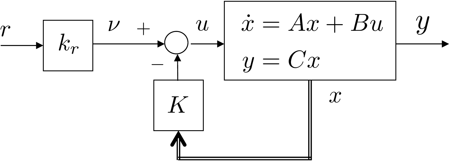
A block diagram of the resulting closed-loop system is shown in Fig. 11.4 where the double line associated with \(x\) is meant to imply that the state \(x\) is not really available. The block diagram also shows the new input \(\nu\). Since the objective is for the output \(y\) to track the reference input \(r\), we let \(\nu(t)=k_r r(t)\), as shown in Fig. 11.4. The feedforward gain \(k_r\) is selected so that the DC gain from \(r\) to \(y\) is equal to one.

From Equation 11.33, the transfer function from \(R\) to \(Y\) is given by \[\tag{11.34} Y(s) = \left(C(sI-(A-BK))^{-1}Bk_r\right) R(s),\] and the DC gain is \[\tag{11.35} k_{DC} = \lim_{s\to 0} \left[C(sI-(A-BK))^{-1}Bk_r\right] = -C(A-BK)^{-1}Bk_r.\] Therefore, the DC gain is equal to one if \[k_r = -\frac{1}{C(A-BK)^{-1}B}.\] The matrix \(A-BK\) will be invertible when there are no eigenvalues at zero. Since \(K\) is selected to place the eigenvalues in the open left half-plane, the matrix will always be invertible, and \(k_r\) exists. Note that in many applications, the output measured by the sensors is not the same as the desired reference output. In other words, the state-space equations may be given by \[\begin{aligned} \dot{x} &= Ax + Bu \\ y_r &= C_r x \\ y_m &= C_m x, \end{aligned}\] where \(y_r\) is the reference output and \(y_m\) is the measured output. In this case, the reference gain \(k_r\) is selected to make the DC gain from \(r\) to \(y_r\) equal to one, or in other words \[\tag{11.36} k_r = -\frac{1}{C_r(A-BK)^{-1}B}.\] Chapter 16 will describe observers that use the measured output \(y_m\) to reconstruct the state \(x\).

The feedforward gain computed in Equation 11.36 is for single input systems. More generally, if the size of the reference output \(y_r\) is equal to the size of the input vector \(u\in\mathbb{R}^m\), then \(C_r\in\mathbb{R}^{m\times n}\) and \(B\in\mathbb{R}^{n\times m}\), which implies that the transfer matrix in Equation 11.34 is square and has dimension \(m\times m\). Similarly, the resulting matrix gain \(K_r\in\mathbb{R}^{m\times m}\) will also be square and from Equation 11.35 will be equal to \[K_r = -\left[C_r(A-BK)^{-1}B\right]^{-1}.\]

11.1.4 State Feedback for Linearized Systems

Suppose that the state-space model is from a linearized system, i.e., suppose that \(x\in\mathbb{R}^n\) is the state and that \(x_e\in\mathbb{R}^n\) is the equilibrium state, and that \(\tilde{x}=x-x_e\) is the state linearized around the equilibrium. Similarly, suppose that \(u\in\mathbb{R}^m\) is the input, that \(u_e\in\mathbb{R}^m\) is the input at equilibrium, and that \(\tilde{u}=u-u_e\) is the input linearized around equilibrium, and that \(y_r\in\mathbf{R}^p\) is the reference output, \(y_{re}=C_rx_e\in\mathbf{R}^p\) is the reference output at equilibrium, and \(\tilde{y}_r=y_r-y_{re}\) is the reference output linearized about equilibrium, then the linearized state-space model is given by \[\begin{aligned} \dot{\tilde{x}} &= A\tilde{x} + B\tilde{u} \\ \tilde{y}_r &= C_r\tilde{x}. \end{aligned}\] Now suppose that the state feedback design process is used to find the state feedback controller \[\tag{11.37} \tilde{u} = -K\tilde{x} + k_r \tilde{r}\] where \(\tilde{r}=r-y_{re}\) is the reference input around the equilibrium output, and where the eigenvalues of \((A-BK)\) are in the open left half-plane, and the DC gain from \(\tilde{r}\) to \(\tilde{y}_r\) is one. The controller input to the plant is therefore \[\tag{11.38} u = u_e - K(x-x_e) + k_r(r-y_{re}).\]

11.2 Summary of Design Process - State Feedback

The state feedback design process can be summarized as follows.

Given the plant \[\begin{aligned} \dot{x} &= Ax + Bu \\ y_r &= C_rx \end{aligned}\] and the desired pole locations \(p_1, p_2, \dots, p_n\), find the gains \(K\) and \(k_r\) so that the feedback controller \[u = -Kx + k_r r\] places the poles at the desired location and results in a DC gain equal to one.

Step 1.
Check to see if the system is controllable by computing the controllability matrix \[\mathcal{C}_{A,B} = [B, AB, \dots, A^{n-1}B]\] and checking to see if \(\text{rank}(\mathcal{C})=n\).

Step 2.
Find the open-loop characteristic polynomial \[\Delta_{ol}(s)=\text{det}(sI-A) = s^n + a_{n-1}s^{n-1} + \cdots + a_1 s + a_0,\] and construct the row vector \[\mathbf{a}_A = (a_{n-1}, a_{n-2}, \dots, a_1, a_0)\] and the matrix \[\mathcal{A}_A = \begin{pmatrix} 1 & a_{n-1} & a_{n-2} & \cdots & a_2 & a_1 \\ 0 & 1 & a_{n-1} & \cdots & a_3 & a_2 \\ \cdots & & \ddots & & & \vdots \\ 0 & 0 & \cdots & 0 & 1 & a_{n-1} \\ 0 & 0 & \cdots & 0 & 0 & 1 \end{pmatrix}\]

Step 3.
Select the desired closed-loop polynomial \[\begin{aligned} \Delta_{cl}^d(s) &= (s-p_1)(s-p_2)\cdots(s-p_n) \\ &= s^n + \alpha_{n-1}s^{n-1} + \cdots + \alpha_1 s + \alpha_0, \end{aligned}\] and construct the row vector \[\boldsymbol{\alpha} = (\alpha_{n-1}, \alpha_{n-2}, \dots, \alpha_1, \alpha_0).\]

Step 4.
Compute the desired gains as \[\begin{aligned} K &= (\boldsymbol{\alpha}-\mathbf{a}_A)\mathcal{A}_A^{-1}\mathcal{C}_{A,B}^{-1} \\ k_r &= \frac{-1}{C_r(A-BK)^{-1}B}. \end{aligned}\]

Using Python, these steps can be implemented as follows:

import control as cnt
import numpy as np

CC = cnt.ctrb(A,B)

# check for controllability
if np.linalg.matrix_rank(CC) == np.size(A,1):
    print('the system is controllable')
else:
    print('the system is not controllable')

# place the poles at p1, p2, ..., pn
K = cnt.place(A, B, [p1, p2, p3])

# compute reference gain
kr = -1/(C @ np.linalg.inv(A - B @ K) @ B)

11.2.1 Simple example

Given the system \[\begin{aligned} \dot{x} &= \begin{pmatrix} 0 & 1 \\ 2 & 3 \end{pmatrix} x + \begin{pmatrix} 0 \\ 4 \end{pmatrix} u \\ y_r &= \begin{pmatrix} 5 & 0 \end{pmatrix} x \end{aligned}\] find the feedback gain \(K\) to place the closed-loop poles at \(-1\pm j\), and the reference gain \(k_r\) so that the DC gain is one.

Step 1.
The controllability matrix is given by \[\mathcal{C}_{A,B} = [B, AB] = \begin{pmatrix} 0 & 4 \\ 4 & 12 \end{pmatrix}.\] The determinant is \(\det(\mathcal{C})=-16\neq 0\), therefore the system is controllable.

Step 2.
The open-loop characteristic polynomial is \[\Delta_{ol}(s)=\det(sI-A) = \det\begin{pmatrix} s & -1 \\ -2 & s-3 \end{pmatrix} = s^2 - 3s -2,\] which implies that \[\begin{aligned} \mathbf{a}_A &= (-3, -2) \\ \mathcal{A}_A &= \begin{pmatrix} 1 & -3 \\ 0 & 1 \end{pmatrix} \end{aligned}\]

Step 3.
The desired closed-loop polynomial is \[\Delta_{cl}^d(s) = (s+1-j)(s+1+j)=s^2+2s+2,\] which implies that \[\boldsymbol{\alpha} = \begin{pmatrix}2, & 2\end{pmatrix}.\]

Step 4.
The gains are therefore given as \[\begin{aligned} K &= (\boldsymbol{\alpha}-\mathbf{a}_A)\mathcal{A}_A^{-1}\mathcal{C}_{A,B}^{-1} \\ &= \left( (2, 2) - (-3, -2) \right)\begin{pmatrix}1 & 3 \\ 0 & 1\end{pmatrix}\begin{pmatrix}-\frac{3}{4} & \frac{1}{4} \\ \frac{1}{4} & 0 \end{pmatrix} \\ &= \begin{pmatrix} 5 & 4 \end{pmatrix} \begin{pmatrix} 0 & \frac{1}{4} \\ \frac{1}{4} & 0 \end{pmatrix} \\ &= \begin{pmatrix} 1 & \frac{5}{4} \end{pmatrix} \end{aligned}\] \[\begin{aligned} k_r &= \frac{-1}{C_r(A-BK)^{-1}B} \\ &= \frac{-1}{\begin{pmatrix} 5 & 0 \end{pmatrix}\left(\begin{pmatrix}0 & 1 \\ 2 & 3\end{pmatrix}-\begin{pmatrix} 0 \\ 4 \end{pmatrix}\begin{pmatrix} 1 & \frac{5}{4}\end{pmatrix}\right)^{-1}\begin{pmatrix} 0 \\ 4 \end{pmatrix}} \\ &= \frac{-1}{\begin{pmatrix} 5 & 0 \end{pmatrix}\left(\begin{pmatrix}0 & 1 \\ 2 & 3\end{pmatrix}-\begin{pmatrix} 0 & 0 \\ 4 & 5 \end{pmatrix}\right)^{-1}\begin{pmatrix} 0 \\ 4 \end{pmatrix}} \\ &= \frac{-1}{\begin{pmatrix} 5 & 0 \end{pmatrix}\begin{pmatrix}0 & 1 \\ -2 & -2\end{pmatrix}^{-1}\begin{pmatrix} 0 \\ 4 \end{pmatrix}} \\ &= \frac{-1}{-10} = \frac{1}{10}. \end{aligned}\]

11.3 Design Study A. Single Link Robot Arm

11.3.1 Example Problem 3.1.14

The objective of this problem is to implement a state feedback controller using the full state. Start with the simulation files developed in Homework 3.1.13.

(a) Select the closed-loop poles as the roots of the equation \(s^2 + 2\zeta\omega_n + \omega_n^2 = 0\), where \(t_r = 0.4890\) and \(\zeta = 0.707\). These values may be different from the parameters found in Homework 3.1.11.

(b) Add the state-space matrices \(A\), \(B\), \(C\), \(D\) derived in Homework 3.1.9 to your param file.

(c) Verify that the state-space system is controllable by checking that \(\text{rank}(\mathcal{C}_{A,B})=n\).

(d) Find the feedback gain \(K\) so that the eigenvalues of \((A-BK)\) are equal to the desired closed-loop poles. Find the reference gain \(k_r\) so that the DC gain from \(\theta_r\) to \(\theta\) is equal to one. Note that if you used the exact same pole values from Homework 3.1.11, \(K=(k_p, k_d)\) where \(k_p\) and \(k_d\) are the proportional and derivative gains found in that problem. Why?

(e) Modify the control code to implement the state feedback controller. Assume that you have access to the entire state.

# 3rd-party
import numpy as np
import control as cnt

# local (controlbook)
from . import params as P
from ..common.controller_base import ControllerBase


class ArmSSController(ControllerBase):
    def __init__(self):
        # tuning parameters
        tr = 0.489
        zeta = 0.707

        # check controllability
        if np.linalg.matrix_rank(cnt.ctrb(P.A, P.B)) != 2:
            raise ValueError("System not controllable")

        # compute gains
        wn = 2.2 / tr  # assumes zeta = 0.707
        des_char_poly = [1, 2 * zeta * wn, wn**2]
        des_poles = np.roots(des_char_poly)
        self.K = cnt.place(P.A, P.B, des_poles)
        self.kr = -1.0 / (P.Cr @ np.linalg.inv(P.A - P.B @ self.K) @ P.B)
        print("des_poles:", des_poles)
        print("K:", self.K)
        print("kr:", self.kr)

        # linearization point
        self.x_eq = P.x_eq
        self.r_eq = P.Cr @ self.x_eq

        # dirty derivative variables
        sigma = 0.05  # cutoff freq for dirty derivative
        self.beta = (2 * sigma - P.ts) / (2 * sigma + P.ts)
        self.thetadot_hat = P.thetadot0
        self.theta_prev = P.theta0

    def update_with_measurement(self, r, y):
        raise NotImplementedError("This controller only uses state feedback.")

    def update_with_state(self, r, x):
        # convert to linearization (tilde) variables
        x_tilde = x - self.x_eq
        r_tilde = r - self.r_eq

        # compute state feedback control
        u_tilde = -self.K @ x_tilde + self.kr @ r_tilde

        # convert back to original variables (feedback linearization)
        theta = x[0]
        u_fl = P.m * P.g * P.ell / 2 * np.cos(theta)
        u_unsat = u_tilde + u_fl
        u = self.saturate(u_unsat, u_max=P.tau_max)
        return u

11.4 Design Study B. Inverted Pendulum

11.4.1 Example Problem 3.2.14

The objective of this problem is to implement a state feedback controller using the full state. Start with the simulation files developed in Homework 3.2.13.

(a) Find the desired closed-loop poles using the values for \(\zeta_z=\zeta_\theta=0.9\), and tune rise times based on the following \(t_z=5 t_{\theta}\).

(b) Add the state-space matrices \(A\), \(B\), \(C\), \(D\) derived in Homework 3.2.9 to your param file.

(c) Verify that the state-space system is controllable by checking that: \(\text{rank}(\mathcal{C})=n\).

(d) Find the feedback gain \(K\) so that the eigenvalues of \((A-BK)\) are equal to the desired closed-loop poles. Find the reference gain \(k_r\) so that the DC gain from \(z_r\) to \(z\) is equal to one.

(e) Implement the state feedback scheme and tune the closed-loop poles to get a good response. You should be able to get a much faster response using state-space methods.

# 3rd-party
import numpy as np
import control as cnt

# local (controlbook)
from . import params as P
from ..common.controller_base import ControllerBase


class CartPendulumSSController(ControllerBase):
    def __init__(self):
        # tuning parameters
        # tr_theta = 0.5  # value before tuning for rise time
        tr_theta = 0.4  # anything faster causes instability due to unmodeled nonlinear dynamics,
        # could also play with "M" to see if that helps.
        zeta_theta = 0.9
        M = 5
        tr_z = tr_theta * M
        zeta_z = 0.9

        # check controllability
        if np.linalg.matrix_rank(cnt.ctrb(P.A, P.B)) != 4:
            raise ValueError("System not controllable")

        # compute gains
        wn_theta = 0.5 * np.pi / (tr_theta * np.sqrt(1 - zeta_theta**2))
        theta_char_poly = [1, 2 * zeta_theta * wn_theta, wn_theta**2]
        theta_poles = np.roots(theta_char_poly)

        wn_z = 0.5 * np.pi / (tr_z * np.sqrt(1 - zeta_z**2))
        z_char_poly = [1, 2 * zeta_z * wn_z, wn_z**2]
        z_poles = np.roots(z_char_poly)

        des_poles = np.hstack([theta_poles, z_poles])

        self.K = cnt.place(P.A, P.B, des_poles)
        self.kr = -1.0 / (P.Cr @ np.linalg.inv(P.A - P.B @ self.K) @ P.B)
        print("des_poles:", des_poles)
        print("K:", self.K)
        print("kr:", self.kr)

        # linearization point
        self.x_eq = P.x_eq
        self.r_eq = P.Cr @ self.x_eq
        self.u_eq = P.u_eq

        # dirty derivative variables
        sigma = 0.05  # cutoff freq for dirty derivative
        self.beta = (2 * sigma - P.ts) / (2 * sigma + P.ts)
        self.zdot_hat = P.zdot0
        self.z_prev = P.z0
        self.thetadot_hat = P.thetadot0
        self.theta_prev = P.theta0

    def update_with_measurement(self, r, y):
        raise NotImplementedError("This controller only uses state feedback.")

    def update_with_state(self, r, x):
        # convert to linearization (tilde) variables
        x_tilde = x - self.x_eq
        r_tilde = r - self.r_eq

        # compute state feedback control
        u_tilde = -self.K @ x_tilde + self.kr @ r_tilde

        # convert back to original variables
        u_unsat = u_tilde + self.u_eq
        u = self.saturate(u_unsat, u_max=P.force_max)
        return u

11.5 Design Study C. Satellite Attitude Control

11.5.1 Example Problem 3.3.14

The objective of this problem is to implement a state feedback controller using the full state. Start with the simulation files developed in Homework 3.3.13.

(a) Using the values for \(\omega_{n_\phi}\), \(\zeta_\phi\), \(\omega_{n_{\theta}}\), and \(\zeta_{\theta}\) selected in Homework 3.3.11, find the desired closed-loop poles.

(b) Add the state-space matrices \(A\), \(B\), \(C\), \(D\) derived in Homework 3.3.9 to your param file.

(c) Verify that the state-space system is controllable by checking that \(\text{rank}(\mathcal{C}_{A,B})=n\).

(d) Find the feedback gain \(K\) so that the eigenvalues of \((A-BK)\) are equal to the desired closed-loop poles. Find the reference gain \(k_r\) so that the DC gain from \(\phi_r\) to \(\phi\) is equal to one.

(e) Implement the state feedback scheme and tune the closed-loop poles to get a good response. You should be able to get a much faster response using state-space methods.

# 3rd-party
import numpy as np
import control as cnt

# local (controlbook)
from . import params as P
from ..common.controller_base import ControllerBase


class SatelliteSSController(ControllerBase):
    def __init__(self):
        # tuning parameters
        tr_theta = 2.0
        zeta_theta = 0.9
        M = 3  # time separation factor between inner and outer loop
        tr_phi = tr_theta * M
        zeta_phi = 0.9

        # check controllability
        if np.linalg.matrix_rank(cnt.ctrb(P.A, P.B)) != 4:
            raise ValueError("System not controllable")

        # compute gains
        wn_theta = 0.5 * np.pi / (tr_theta * np.sqrt(1 - zeta_theta**2))
        theta_char_poly = [1, 2 * zeta_theta * wn_theta, wn_theta**2]
        theta_poles = np.roots(theta_char_poly)

        wn_phi = 0.5 * np.pi / (tr_phi * np.sqrt(1 - zeta_phi**2))
        phi_char_poly = [1, 2 * zeta_phi * wn_phi, wn_phi**2]
        phi_poles = np.roots(phi_char_poly)

        des_poles = np.hstack([theta_poles, phi_poles])

        self.K = cnt.place(P.A, P.B, des_poles)
        self.kr = -1.0 / (P.Cr @ np.linalg.inv(P.A - P.B @ self.K) @ P.B)
        print("des_poles:", des_poles)
        print("K:", self.K)
        print("kr:", self.kr)

        # linearization point
        self.x_eq = P.x_eq
        self.r_eq = P.Cr @ self.x_eq
        self.u_eq = P.u_eq

        # dirty derivative variables
        sigma = 0.05  # cutoff freq for dirty derivative
        self.beta = (2 * sigma - P.ts) / (2 * sigma + P.ts)
        self.thetadot_hat = P.thetadot0
        self.theta_prev = P.theta0
        self.phidot_hat = P.phidot0
        self.phi_prev = P.phi0

    def update_with_measurement(self, r, y):
        raise NotImplementedError("This controller only uses state feedback.")

    def update_with_state(self, r, x):
        # convert to linearization (tilde) variables
        x_tilde = x - self.x_eq
        r_tilde = r - self.r_eq

        # compute state feedback control
        u_tilde = -self.K @ x_tilde + self.kr @ r_tilde

        # convert back to original variables
        u_unsat = u_tilde + self.u_eq
        u = self.saturate(u_unsat, u_max=P.torque_max)
        return u

11.6 Interactive State-Feedback Check

11.7 Coding Lab: Full-State Feedback

11.8 Knowledge Check

11.9 Notes and References

Controllability is typically defined as follows. The state-space system \[\dot{x}=Ax+Bu\] is said to be controllable from initial state \(x_0\), if there exists a control function \(u(t)\) defined on some interval \(t\in[0,T]\) that transitions the state to the origin. It can be shown that for linear time-invariant systems, the system is controllable if and only if the rank of the controllability matrix \(\mathcal{C}_{A,B}\) is equal to the size of the state \(n\). For single input systems, this is equivalent to \(\mathcal{C}_{A,B}\) being invertible. Controllability is an interesting and deep topic that extends nicely to nonlinear and multi-input systems. For further information see [5, 6, 12].

Ackermann’s formula given in Equation 11.32 is only valid for single input systems. In the multi-input case, the controllability matrix \(\mathcal{C}_{A,B}\) is not square and therefore cannot be inverted. However, a more general formula can be derived if \(\mathcal{C}_{A,B}\) has rank \(n\). The more general formula is implemented by the place command in both MATLAB and Python. For additional information on the derivation of the feedback gain in the MIMO case see [6].