1 Introduction

Introduction

Overview

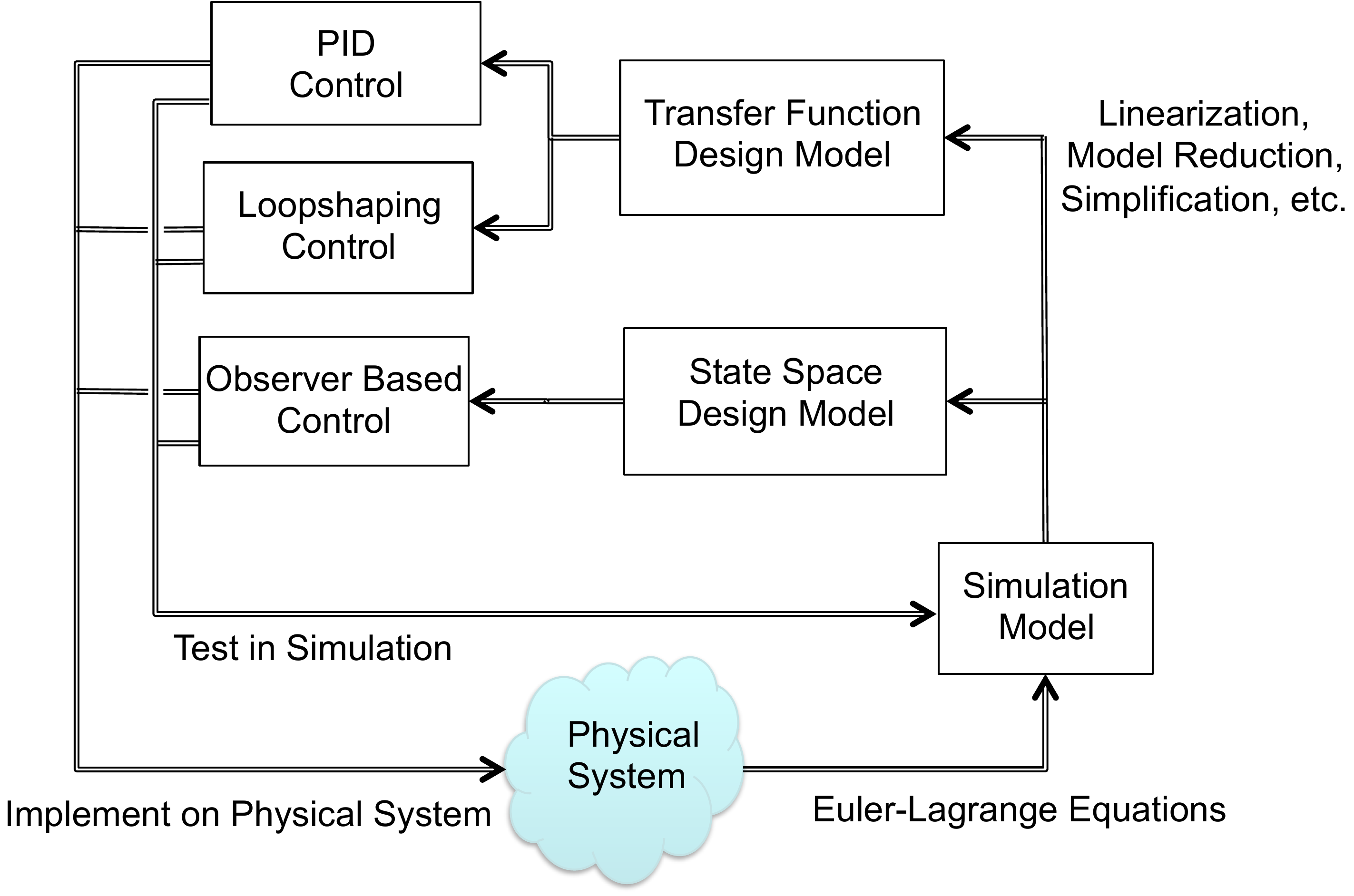
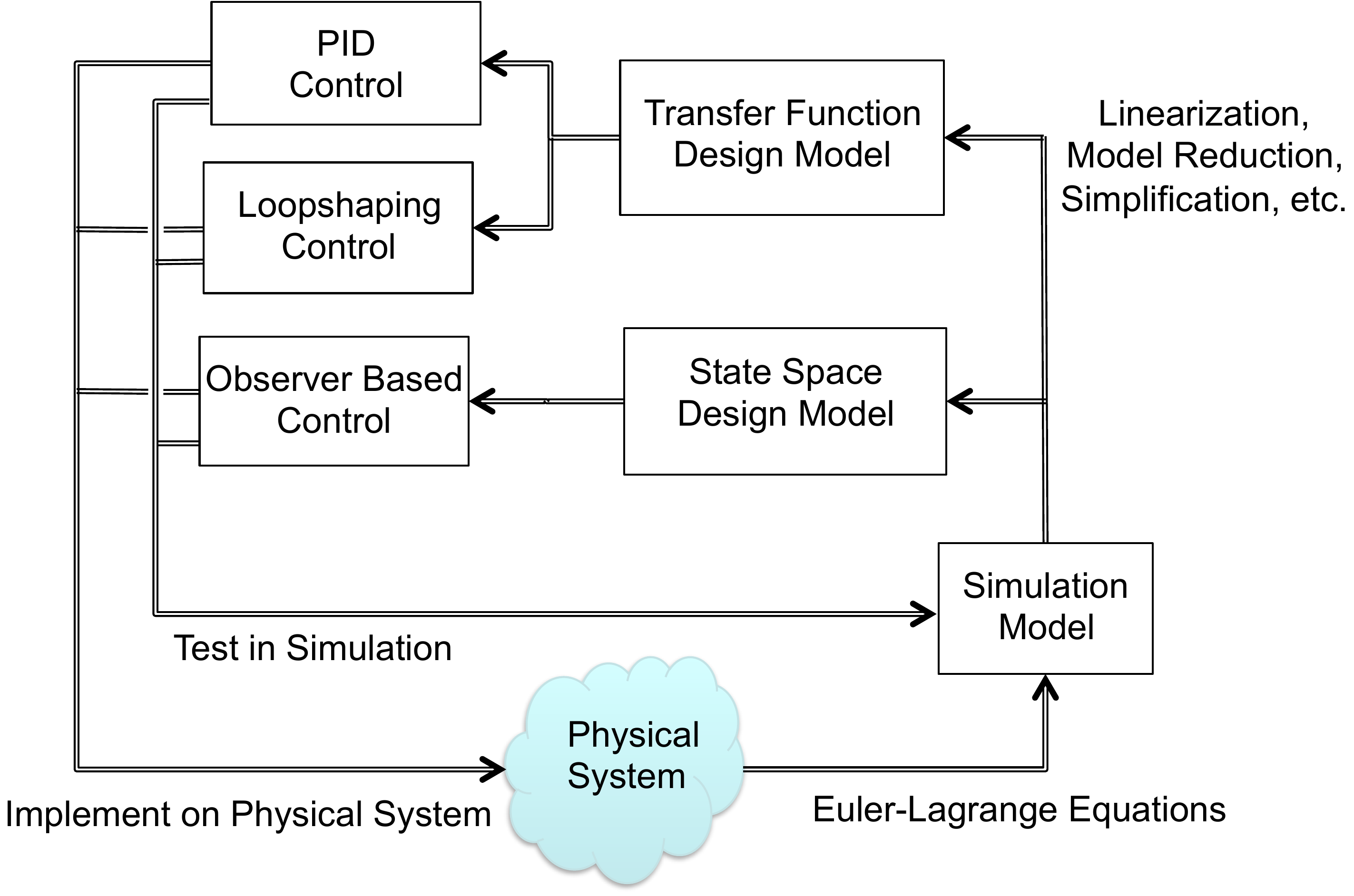
The objective of this book is to prepare the reader to design feedback control systems for dynamic systems and to lay the groundwork for further studies in the area. The design philosophy that we follow throughout the book is illustrated schematically in Fig. 1.1. The objective is to design a control system for the “Physical System” shown in Fig. 1.1. The physical system includes actuators like motors and propellers, and sensors like accelerometers, gyros, GPS, cameras, and pressure sensors. The first step in the design process is to model the physical system using nonlinear differential equations. While approximations and simplifications will be necessary at this step, the hope is to capture, in mathematics, all of the important characteristics of the physical system. While there are many different methods for developing the equations of motion of the physical systems, in this book we will introduce one specific method, the Euler-Lagrange method, that is applicable to a wide variety of mechanical systems. We will, for the most part, abstract the actuators to applied forces and torques on the system. Similarly, the sensors will be abstracted to general measurements of certain physical quantities like position and velocity. The resulting model is called the Simulation Model as shown in Fig. 1.1. In the design process, the simulation model is used for the high fidelity computer simulation of the physical system. Every control design will be tested thoroughly on the simulation model. However, the simulation model is only a mathematical approximation of the physical system, and simply because a design is effective on the simulation model, we should not assume that it will function properly on the physical system. Part I of the book introduces the Euler-Lagrange method and demonstrates how to derive simulation models for mechanical systems using this method.

1.1 Interactive Control Workflow

Click Figure 1.1

The diagram below is the same design-process figure, but the major regions are clickable. Select a region to see how that part of the workflow will be developed later in the book.

Physical system Simulation model Transfer-function design model State-space design model Control design methods Test in simulation Implementation

The simulation model is typically nonlinear and high order and is too mathematically complex to be useful for control design. Therefore, to facilitate design, the simulation model is simplified and usually linearized to create lower-order design models. For any physical system, there may be multiple design models that capture certain aspects of the system that are important for a particular design. In this book we will introduce the two most common design models used for control systems analysis and design: transfer-function models and state-space models. In both cases we will linearize the system about a particular operating condition. The advantage of transfer function models is that they capture the frequency dependence of the input-output relationship in dynamic systems. The advantage of state-space models is that they are more intuitive and are better adapted to numerical implementation. Part II of the book shows how to linearize the equations of motion and how to create transfer function and state-space design models.

The next three parts, Part III–V, introduce three different control design methods. Part III shows how to design Proportional-Integral-Derivative (PID) controllers for second-order systems. The PID method is the most common control technique used in industry. It can be understood from both a time-domain and frequency-domain perspective. The advantage of PID is its simplicity in design and implementation and the fact that it can be used to achieve high performance for a surprising variety of systems. However, the disadvantage of PID control is that stability and performance can typically only be guaranteed for second-order systems. Therefore, Part III is focused exclusively on second-order systems.

In Part IV we introduce the observer-based control method. Observer-based methods can be thought of as a natural extension of PID controllers to higher-order systems. However, observer-based methods are much more general than PID and can be used to obtain higher performance. In addition, most observer-based techniques extend to nonlinear and time-varying systems. The disadvantages of observer-based methods are that they require a higher level of mathematical sophistication to understand and use, and they are primarily time-domain methods.

The final design technique, which is covered in Part V, is the loop shaping control design method. The loop shaping method is a frequency domain technique that explicitly addresses robustness of the system. The loop shaping method is also a natural extension of PID control to higher-order systems. One of the advantages of loop shaping techniques is that they can be used when only a frequency response model of the system is available.

The book is organized around several design studies. For each new concept that is introduced, we will apply that concept to three specific design problems. The design problems are introduced in the following three sections and include a single-link robot arm, a pendulum on a cart, and a simple satellite attitude control problem. The homework problems, which are provided in Part VI, will follow the same format with problems that are identical to those worked in the book, but they will be applied to different physical systems. Our hope is to illustrate the control design process with specific, easy-to-understand problems. We note, however, that the concepts introduced in this book are applicable to a much wider variety of problems than those illustrated in the book. We focus on mechanical systems, but a similar process (with the exception of the modeling section) can be followed for any system that can be modeled using ordinary differential equations. Examples include aerodynamic systems, electrical systems, chemical processes, large structures like buildings and bridges, biological feedback systems, economic systems, queuing systems, and many more.

1.2 Design-Study Preview

1.3 Design Studies

1.3.1 Design Study: Single Link Robot Arm

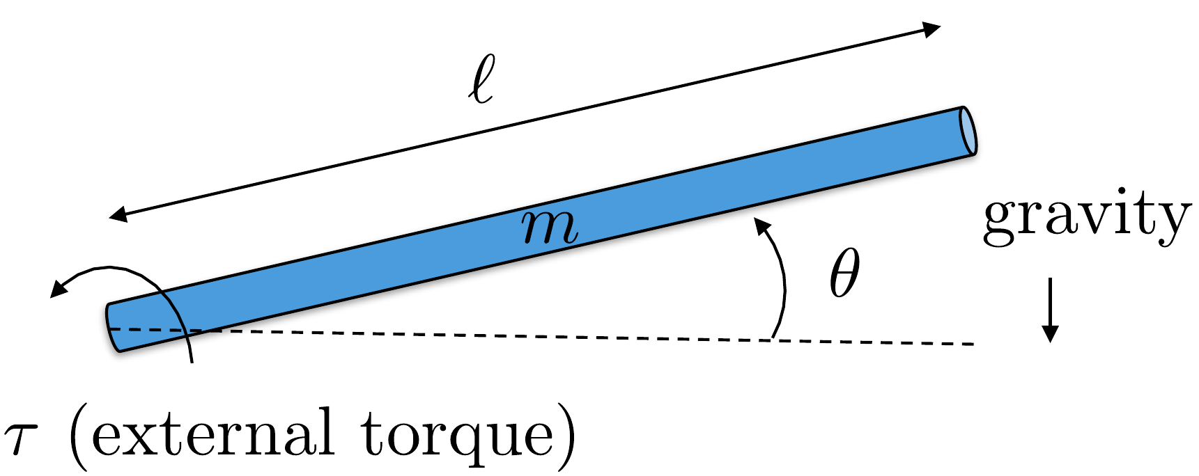
Figure 1.2 shows a single-link robot arm system. The robot arm has mass \(m\) and length \(\ell\). The angle of the robot is given by \(\theta\) as measured from horizontal to the ground. The angular speed of the arm is \(\dot{\theta}\). There is an applied torque \(\tau\) at the joint. There is also a damping (or viscous friction) torque that opposes the rotation of the joint and which can be modeled as \(-b\dot{\theta}\).

The actual physical parameters of the system are \(m=0.5\) kg, \(\ell=0.3\) m, \(g=9.8\) m/s\(^2\), \(b=0.01\) Nms. The torque is limited by \(\left|\tau\right|\leq 1\) Nm.

A.2 Kinetic energy.

A.3 Equations of motion.

A.4 Linearize equations of motion.

A.5 Transfer function model.

A.6 State-space model.

A.7 Pole placement using PD.

A.8 Second-order design.

A.9 Integrators and system type.

A.P.6 Root locus.

A.10 Digital PID.

A.11 Full state feedback.

A.12 Full state with integrator.

A.13 Observer based control.

A.14 Disturbance observer.

A.15 Frequency response.

A.16 Loop gain.

A.17 Stability margins.

A.18 Loopshaping design.

Note: The notation identifies the design configuration and the chapter in which it is used: Example A.4 refers to the application of approximations in Chapter 4 to linearize design configuration A. Similarly, Example A.P.6 refers to the root locus assignment associated with Appendix A.P.6.

1.3.2 Design Study: Pendulum on a Cart

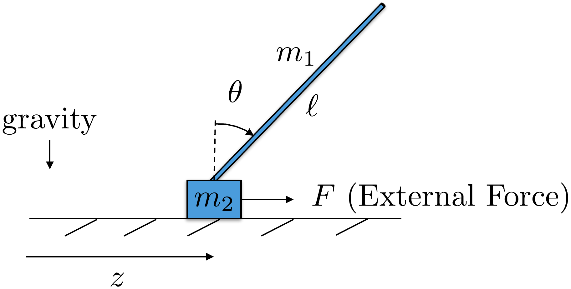
Figure 1.3 shows the pendulum on a cart system, also called an inverted pendulum. The position of the cart measured from the origin is \(z\) and the linear speed of the cart is \(\dot{z}\). The angle of the pendulum from straight up is given by \(\theta\), and the angular velocity is \(\dot{\theta}\). The rod is of length \(\ell\), and has mass \(m_1\), and is approximated as being infinitely thin. The cart has mass \(m_2\). Gravity acts in the down direction. The only applied force is \(F\), which acts in the direction of \(z\). The cart slides on a frictionless surface, but air friction produces a damping force equal to \(-b\dot{z}\).

The physical constants are \(m_1=0.25\) kg, \(m_2=1.0\) kg, \(\ell=1.0\) m, \(g=9.8\) m/s\(^2\), \(b=0.05\) Ns. The force is limited by \(\left|F\right|\leq 5\) N.

B.2 Kinetic energy.

B.3 Equations of Motion.

B.4 Linearize equations of motion.

B.5 Transfer function model.

B.6 State-space model.

B.8 Successive loop closure.

B.9 Integrators and system type.

B.P.6 Root locus.

B.10 Digital PID.

B.11 Full state feedback.

B.12 Full state with integrator.

B.13 Observer based control.

B.14 Disturbance observer.

B.15 Frequency Response.

B.16 Loop gain.

B.17 Stability margins.

B.18 Loopshaping design.

1.3.3 Design Study: Satellite Attitude Control

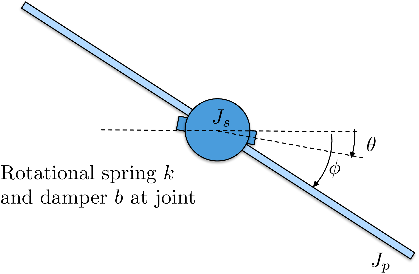
Figure 1.4 shows a simplified version of a satellite with flexible solar panels. We will model the flexible panels using a rigid sheet with moment of inertia \(J_p\) connected to the main satellite body by a torsional compliant element with spring constant \(k\) and damping constant \(b\). The moment of inertia of the satellite is \(J_s\). The angle of the satellite body from the inertial reference is \(\theta\) and the angle of the panel from the inertial reference is denoted as \(\phi\). Thrusters are used to command an external torque of \(\tau\) about the axis of the satellite body.

The physical constants are \(J_s=5\) kg m\(^2\), \(J_p=1\) kg m\(^2\), \(k=0.1\) N m, \(b=0.05\) Nms. The torque is limited by \(\left|\tau\right|\leq 5\) Nm.

C.2 Kinetic energy.

C.3 Equations of motion.

C.4 Equilibria.

C.5 Transfer function model.

C.6 State-space model.

C.8 Successive loop closure.

C.9 Integrators and system type.

C.P.6 Root locus.

C.10 Digital PID.

C.11 Full state feedback.

C.12 Full state with integrator.

C.13 Observer based control.

C.14 Disturbance observer.

C.15 Frequency Response.

C.16 Loop gain.

C.17 Stability margins.

C.18 Loopshaping design.

1.4 Knowledge Check

Use these quick checks to test the Chapter 1 workflow vocabulary before moving on. The short-answer checks are intentionally limited to terms that can be graded reliably.