In the previous chapter we derived a full state feedback controller
that stabilized the system and ensured that the DC gain from the
reference \(r(t)\) to the reference
output \(y_r(t)\) is equal to one. If the model is
precise, meaning that we know all of the parameters exactly and we have
not neglected any dynamics, or if there are no disturbances on the
system, then the output will track the reference as time goes to
infinity. However, models are never precise, and there are almost always
disturbances on the system, which implies that there will be
steady-state error in the response. In
Chapter 12 we showed that adding an
integrator to the controller is an effective way of eliminating
steady-state error caused by model mismatch and input/output
disturbances. In this section we will show how to add an integrator to
the full state feedback controller derived in
Chapter 14.
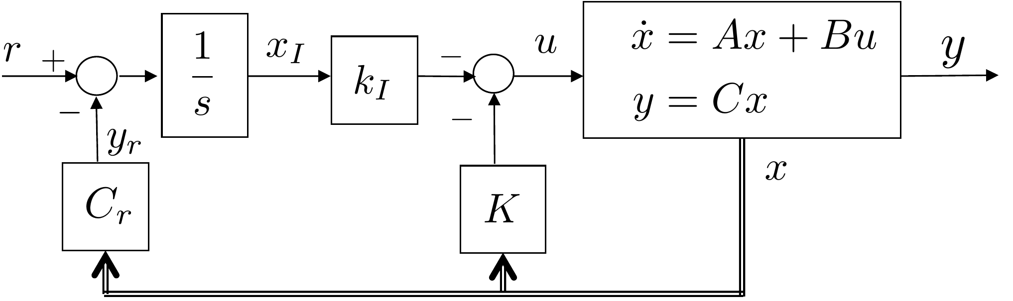
A block diagram of the system with full state feedback and an
integrator is shown in
Fig.12.1.
Figure 12.1. Full state feedback with
integrator.
Let the state of the integrator be defined as \(x_I\), as shown in
Fig.12.1. Then
\[\dot{x}_I = r-y_r = r-C_rx.\] In
Appendix 30 we argue, using the root
locus, that adding an
integrator after the other gains are selected will change all of the
pole locations. Since the pole placement design methods
described in Part III were limited to second-order
systems, we did not have an effective method for placing the system
poles and the integrator pole simultaneously. On the other hand, the
pole placement technique described in
Chapter 14 was not limited to
second-order systems. As such, there should be a way to use the methods
of Chapter 14 to simultaneously place both
the system poles and the integrator pole. To do so, we augment the
states of the original system with the integrator state \(x_I\). Since the dynamics of the original
system are given by \(\dot{x}=Ax+Bu\),
the dynamics of the augmented system are given by \[\tag{12.1}
\begin{pmatrix} \dot{x} \\ \dot{x}_I \end{pmatrix} = \begin{pmatrix} A
& \mathbf{0} \\ -C_r & \mathbf{0}\end{pmatrix} \begin{pmatrix} x
\\ x_I \end{pmatrix} + \begin{pmatrix} B \\ \mathbf{0} \end{pmatrix} u +
\begin{pmatrix} 0 \\ 1 \end{pmatrix} r,\] where the state of the
augmented system is \((x^\top, x_I)^\top\), the interaction
matrix, or the “\(A\)-matrix,” of the augmented system is
\[A_1 = \begin{pmatrix} A & \mathbf{0} \\
-C_r & \mathbf{0}\end{pmatrix},\] and the “\(B\)-matrix” of the augmented system is
\[B_1=\begin{pmatrix} B \\
\mathbf{0}\end{pmatrix}.\] The first question that might be asked
is whether the augmented system \((A_1,B_1)\) is controllable when the
original system \((A,B)\) is
controllable. Since the original
system is controllable, we know that the controllability matrix \[\mathcal{C}_{A,B} = \begin{pmatrix} B & AB
& \dots & A^{n-1}B \end{pmatrix}\] has rank \(n\). For the augmented system, the
controllability matrix is \[\mathcal{C}_{A_1,B_1}
= \begin{pmatrix} B & AB & A^2B & \dots & A^{n-1}B &
A^nB \\ 0 & -C_rB & -C_rAB & \dots & -C_rA^{n-2}B &
-C_rA^{n-1}B \end{pmatrix},\] which is guaranteed to have rank
\(n+1\) if \(C_rA^{n-1}B \neq 0\). When the augmented
system is controllable, we can use the pole placement technique
described in
Chapter 14 to place the system poles
and the pole of the integrator simultaneously using the augmented
system. For example, letting \(A_1\)
and \(B_1\) represent the augmented
system, and using the Python place command
import control as cnt
K1 = cnt.place(A1,B1, [p1,...,pn,pI])
where \(p_I\) is the integrator
pole. The resulting controller is \[\begin{aligned}
u(t) &= -K_1\begin{pmatrix}x \\ x_I \end{pmatrix} = -\begin{pmatrix}
K & k_I \end{pmatrix}\begin{pmatrix}x \\ x_I \end{pmatrix}
=-Kx-k_Ix_I\\
&= \underbrace{-Kx(t)}_{\text{state feedback}} - \underbrace{k_I
\int_0^t(r(\tau)-y_r(\tau))d\tau}_{\text{integral feedback}} \quad.
\end{aligned}\]
We can show that adding the integrator ensures that the DC
gain of the closed-loop
system is equal to one. Indeed, from
Equation 12.1 the
augmented closed-loop system is \[\begin{aligned}
\begin{pmatrix} \dot{x} \\ \dot{x}_I \end{pmatrix} &=
\begin{pmatrix} A & \mathbf{0} \\ -C_r & \mathbf{0}\end{pmatrix}
\begin{pmatrix} x \\ x_I \end{pmatrix} - \begin{pmatrix} B \\ \mathbf{0}
\end{pmatrix} \begin{pmatrix} K & k_I \end{pmatrix}\begin{pmatrix} x
\\ x_I \end{pmatrix} + \begin{pmatrix} 0 \\ 1 \end{pmatrix} r \\
&= \begin{pmatrix} A-BK & -Bk_I \\ -C_r &
0\end{pmatrix}\begin{pmatrix} x \\ x_I \end{pmatrix} +
\begin{pmatrix} 0 \\ 1 \end{pmatrix} r,
\end{aligned}\] where the reference output equation is \[y_r = \begin{pmatrix} C_r & 0 \end{pmatrix}
\begin{pmatrix} x \\ x_I \end{pmatrix}.\] Therefore, the
transfer function from \(R(s)\) to
\(Y_r(s)\) is \[Y_r(s) = \begin{pmatrix} C_r & 0
\end{pmatrix} \left(sI - \begin{pmatrix} A-BK & -Bk_I \\ -C_r &
0\end{pmatrix}\right)^{-1} \begin{pmatrix} 0 \\ 1 \end{pmatrix}
R(s),\] which implies that the DC gain is \[\begin{aligned}
k_{DC} &= -\begin{pmatrix} C_r & 0
\end{pmatrix} \begin{pmatrix} A-BK & -Bk_I \\ -C_r &
0\end{pmatrix}^{-1} \begin{pmatrix} 0 \\ 1 \end{pmatrix}.
\end{aligned}\] Defining \(M\stackrel{\triangle}{=}(A-BK)^{-1}\), and
using the Matrix inversion formula for block matrices given in
Appendix 31
Equation P.7.2
we get \[\begin{aligned}
k_{DC} &= -\begin{pmatrix} C_r & 0
\end{pmatrix} \begin{pmatrix} M-MBk_I(C_rMBk_I)^{-1}C_rM &
-MBk_I(C_rMBk_I)^{-1} \\ -(C_rMBk_I)^{-1}C_rM &
(C_rMBk_I)^{-1}\end{pmatrix} \begin{pmatrix} 0 \\ 1 \end{pmatrix} \\
&= C_rMBk_I(C_rMBk_I)^{-1} \\
&= 1.
\end{aligned}\]
12.1.1 Integral Feedback for
Linearized Systems
Suppose that the
state-space model is from a linearized system, i.e., suppose that \(x\in\mathbb{R}^n\) is the state, \(x_e\in\mathbb{R}^n\) is the equilibrium
state, and that \(\tilde{x}=x-x_e\) is
the state linearized around the equilibrium. Similarly, suppose that
\(u\in\mathbb{R}^m\) is the input, that
\(u_e\in\mathbb{R}^m\) is the input at
equilibrium, and that \(\tilde{u}=u-u_e\) is the input linearized
around equilibrium, and that \(y_r\in\mathbf{R}^p\) is the reference
output, \(y_{re}=C_rx_e\in\mathbf{R}^p\) is the
reference output at equilibrium, \(\tilde{y}_r=y_r-y_{re}\) is the reference
output linearized about equilibrium, and the reference input is given by
\(\tilde{r}=r-y_{re}\). In this case
the integral state is selected as \(\tilde{x}_I=\int(\tilde{r}-\tilde{y}_r)d\tau\),
and the augmented system is given by \[\begin{pmatrix} \dot{\tilde{x}} \\
\dot{\tilde{x}}_I \end{pmatrix} = \begin{pmatrix} A & \mathbf{0} \\
-C_r & \mathbf{0}\end{pmatrix} \begin{pmatrix} \tilde{x} \\
\tilde{x}_I \end{pmatrix} + \begin{pmatrix} B \\ \mathbf{0}
\end{pmatrix} \tilde{u} + \begin{pmatrix} 0 \\ 1 \end{pmatrix}
\tilde{r}.\] The pole placement design proceeds as in the
previous section with the resulting controller being \[\tilde{u} = -K\tilde{x} - k_I \int_{-\infty}^t
\tilde{e}(\tau)d\tau.\] Noting that \[\tilde{e} = \tilde{r}-\tilde{y} =
(r-y_{re})-(y_r-y_{re}) = r-y_r\] we get that the controller for
the linearized system is given by \[u = u_e -
K(x-x_e) - k_I \int_{-\infty}^t (r(\tau)-y_r(\tau))d\tau.\]
12.2 Summary of Design Process -
State Feedback with Integrator
The design process for adding an integrator to state feedback can be
summarized as follows. Given the plant \[\begin{aligned}
\dot{x} &= Ax + Bu \\
y_r &= C_rx,
\end{aligned}\] where we desire that \(y_r\) tracks the reference \(r\) using integral action using the
controller \[u(t) = -Kx(t) -
k_I\int_{-\infty}^t (r(\tau)-y_r(\tau))d\tau,\] with desired
closed-loop gains at \(p_1, p_2, \dots,
p_n\), \(p_I\).
Step 1.
Augment the state evolution equation as \[\begin{pmatrix}\dot{x} \\ \dot{x}_I \end{pmatrix}
= \begin{pmatrix} A & \mathbf{0} \\ -C_r & \mathbf{0}
\end{pmatrix} \begin{pmatrix}x \\ x_I\end{pmatrix} + \begin{pmatrix}B \\
\mathbf{0}\end{pmatrix}u + \begin{pmatrix}\mathbf{0} \\
I\end{pmatrix}r,\] and let \[\begin{aligned}
A_1 &= \begin{pmatrix} A & \mathbf{0} \\ -C_r & \mathbf{0}
\end{pmatrix} \\
B_1 &= \begin{pmatrix}B \\ \mathbf{0}\end{pmatrix}
\end{aligned}\]
Step 2.
Follow the pole placement procedure outlined in
Chapter 14 to find \(K_1\) that places the poles of the
augmented system at \(p_1, p_2, \dots,
p_n\), and \(p_I\).
Step 3.
Find the gains \(K\) and \(k_I\) as \[\begin{aligned}
K &= K_1(1:n) \\
k_I &= K_1(n+1).
\end{aligned}\]
Using Python, these steps can be implemented using the following
script.
import numpy as np
import control as cnt

# augment the system matrices
A1 = np.vstack((
    np.hstack((A, np.zeros((np.size(A,1),1)))),
    np.hstack((-Cr, 0)) ))

B1 = np.vstack((
    B, 0))

# Compute the gains if the system is controllable
if np.linalg.matrix_rank(cnt.ctrb(A1, B1)) != np.size(A1,1):
    print("The system is not controllable")
else:
    K1 = cnt.acker(A1, B1, [p1, p2, ..., pn, pI])

    #extract the state feedback gains and the integral gain
    K = K1[0,0:-1]
    ki = K1[0,-1]

print('K: ', K)
print('ki: ', ki)
12.2.1 Simple example
Given the system \[\begin{aligned}
\dot{x} &= \begin{pmatrix} 0 & 1 \\ 2 & 3 \end{pmatrix} x +
\begin{pmatrix} 0 \\ 4 \end{pmatrix} u \\
y_r &= \begin{pmatrix} 5 & 0 \end{pmatrix} x
\end{aligned}\] find the feedback gain \(K\) to place the closed-loop poles at \(-1\pm j\), and the reference gain \(k_r\) so that the DC gain is one, and add
an integrator with gain at \(p_I=-0.1\).
Step 2.
To place the poles at \(p_1=-1+j\),
\(p_2=-1-j\), \(p_I=-0.1\), we first form the
controllability matrix \[\mathcal{C}_{A_1,B_1} = [B_1, A_1B_1, A_1^2B_1] =
\begin{pmatrix} 0 & 4 & 12 \\ 4 & 12 & 44 \\ 0 & 0
& -20 \end{pmatrix}.\] The determinant is \(det(\mathcal{C}_{A_1,B_1})=320\neq 0\),
therefore the system is controllable.
Step 3.
The feedback gains are therefore given by \[\begin{aligned}
K &= K_1(1:2) = \begin{pmatrix} 1.05, & 1.275 \end{pmatrix} \\
k_I &= K_1(3) = -0.01
\end{aligned}\]
Alternatively, we could have used the following Python script
import numpy as np
import control as cnt

# define original state-space system and desired poles
A = np.array([[0.0, 1.0], [2.0, 3.0]])
B = np.array([[0.0], [4.0]])
Cr = np.array([5.0, 0])

p1 = -1.0 - 1.j
p2 = -1.0 + 1.j
pI = -0.1

# augment the system matrices
A1 = np.vstack((
    np.hstack((A, np.zeros((np.size(A,1),1)))),
    np.hstack((-Cr, 0)) ))
B1 = np.vstack((
    B, 0))

# Compute the gains if the system is controllable
if np.linalg.matrix_rank(cnt.ctrb(A1, B1)) != np.size(A1,1):
    print("The system is not controllable")
else:
    K1 = cnt.acker(A1, B1, [p1, p2, pI])

    #extract the state feedback gains and the integral gain
    K = K1[0,0:-1]
    ki = K1[0,-1]
Chapter 12 guided activity
Work through a second integrator-augmented design
Use the same procedure as the simple example above. For the system
below, compute each quantity in order and click Check
before moving on. The solution for each step is revealed only after that
step is checked.
Desired augmented closed-loop poles:
-1 and
-2 ± j.
Step 1. Augmented system
Form A1 = (A, 0; -Cr, 0) and B1 = (B;
0). Enter A1 row by row and B1 from top to bottom.
Modify the state feedback solution developed in
Homework 3.1.14 to add an integrator with
anti-windup.
Add a 0.25 Newton disturbance to the system and allow the system
parameters to change up to 20%.
Tune the integrator pole (and other gains if necessary) to get good
tracking performance.
Design Study A guided exercise
Add integral action
Augment the state with the
integral of tracking error and place the added pole deliberately.
Step 1. Augmented system size
Show solution for Step
1
Answer: The two plant states plus
one integrator state give a third-order augmented
model.
Step 2. Integrator pole placement
Show solution for Step
2
Answer: The added integrator pole
must be placed in the stable left half-plane.
Step 3. Gain partition
Show solution for Step
3
Answer: The augmented gain is
separated into the state-feedback gain \(K\) and integral gain \(k_I\).
Pseudocode
The complete solution includes
state-feedback-with-integrator code. Before opening it, outline how you
would update the integrator state, compute the augmented feedback input,
and apply anti-windup if needed.
This prompt is
ungraded. It is intended to connect the augmented-state design to the
implementation code in the complete solution.
Complete solution
Step 1.
The original state-space equations are \[\begin{aligned}
\dot{x} &= \begin{pmatrix} 0 & 1.0000 \\ 0 & -0.667
\end{pmatrix}x + \begin{pmatrix} 0 \\ 66.667 \end{pmatrix} u \\
y &= \begin{pmatrix}1 & 0 \end{pmatrix}x,
\end{aligned}\] therefore the augmented system is \[\begin{aligned}
A_1 &= \begin{pmatrix} A & \mathbf{0} \\ -C & \mathbf{0}
\end{pmatrix} = \begin{pmatrix} 0 & 1.0000 & 0 \\ 0
& -0.667 & 0 \\ -1 & 0 & 0 \end{pmatrix} \\
B_1 &= \begin{pmatrix} B \\ \mathbf{0} \end{pmatrix} =
\begin{pmatrix} 0 \\ 66.667 \\ 0 \end{pmatrix}
\end{aligned}\]
Step 2.
After the design in HW 3.1.14, the closed-loop poles were
located at \(p_{1,2} = -3.18 \pm j
3.18\). We will add the integrator pole at \(p_I=-5\). The new controllability matrix is
\[\begin{aligned}
\mathcal{C}_{A_1,B_1} &= [B_1, A_1B_1, A_1^2B_1] \\ &=
\begin{pmatrix}
0 & 66.6670 & -44.4669 \\
66.6670 & -44.4669 & 29.6594 \\
0 & 0 & -66.6670
\end{pmatrix}.
\end{aligned}\]
The determinant is \(det(\mathcal{C}_{A_1,B_1})=2.9630e+05\neq
0\), therefore the system is controllable.
The desired closed-loop polynomial \[\begin{aligned}
\Delta_{cl}^d(s) &=s^3+11.36s^2+52.04s+101.2,
\end{aligned}\] which implies that \[\boldsymbol{\alpha} = \begin{pmatrix}11.36,
& 52.04, & 101.2\end{pmatrix}.\]
The augmented gains are therefore given as \[\begin{aligned}
K_1 &=
(\boldsymbol{\alpha}-\mathbf{a}_{A_1})\mathcal{A}_{A_1}^{-1}\mathcal{C}_{A_1,B_1}^{-1}
\\
&= \begin{pmatrix} 0.7807, & 0.1604, & -1.518
\end{pmatrix}
\end{aligned}\]
Step 3.
The feedback gains are therefore given by \[\begin{aligned}
K &= K_1(1:2) = \begin{pmatrix} 0.7807, & 0.1604
\end{pmatrix} \\
k_I &= K_1(3) = -1.518
\end{aligned}\]
A Python class that implements state feedback control with an
integrator for the single link robot arm is shown below.
# 3rd-partyimport numpy as npimport control as cnt# local (controlbook)from . import params as Pfrom ..common.controller_base import ControllerBaseclass ArmSSIController(ControllerBase):def__init__(self, separate_integrator=True):# tuning parameters tr =0.489 zeta =0.707 integrator_pole = [-5.0]# augmented system A1 = np.block([[P.A, np.zeros((2, 1))], [-P.Cr, np.zeros(1)]]) B1 = np.vstack((P.B, 0))# check controllabilityif np.linalg.matrix_rank(cnt.ctrb(A1, B1)) !=3:raiseValueError("System not controllable")# compute gains wn =2.2/ tr # assumes zeta = 0.707 des_char_poly = [1, 2* zeta * wn, wn**2] des_sys_poles = np.roots(des_char_poly) des_poles = np.hstack((des_sys_poles, integrator_pole))self.K1 = cnt.place(A1, B1, des_poles)self.K =self.K1[:, :2]self.ki =self.K1[:, 2:]print("des_poles:", des_poles)print("K1:", self.K1)print("K:", self.K)print("ki:", self.ki)# linearization pointself.x_eq = P.x_eqself.r_eq = P.Cr @self.x_eqself.x1_eq = np.hstack((self.x_eq, 0))# dirty derivative variables sigma =0.05# cutoff freq for dirty derivativeself.beta = (2* sigma - P.ts) / (2* sigma + P.ts)self.thetadot_hat = P.thetadot0self.theta_prev = P.theta0# integrator variablesself.error_prev =0.0self.error_integral =0.0self.separate_integrator = separate_integratordef update_with_measurement(self, r, y):raiseNotImplementedError("This controller only uses state feedback.")def update_with_state(self, r, x):# convert to linearization (tilde) variables x_tilde = x -self.x_eq# integrate error error = r - P.Cr @ x # can also use tilde vars (eq subtracts out)self.error_integral += P.ts * (error +self.error_prev) /2self.error_prev = error# compute feedback controlifself.separate_integrator: u_tilde =-self.K @ x_tilde -self.ki @self.error_integralelse: x1_tilde = np.hstack((x_tilde, self.error_integral)) u_tilde =-self.K1 @ x1_tilde# convert back to original variables (feedback linearization) theta = x[0] u_fl = P.m * P.g * P.ell /2* np.cos(theta) u_unsat = u_tilde + u_fl u =self.saturate(u_unsat, u_max=P.tau_max)return u
Complete simulation code for MATLAB, Python, and Simulink can be
downloaded at http://controlbook.byu.edu.
(a) Modify the state feedback solution developed in
Homework 3.2.14 to add an integrator with
anti-windup to the position feedback.
(b) Add a constant input disturbance of 0.5 Newtons to the input of the
plant and allow the system parameters to change up to 20%.
(c) Tune the integrator pole (and other gains if necessary) to get good
tracking performance. You may need to make the gains less aggressive
(slower rise time) to get stable performance.
Design
Study B guided exercise
Add cart-position integral
action
Augment the system with an integrator on z tracking
error.
Step 1. Integrated
output
Show solution for Step
1
Answer: The integrator is added
to cart-position tracking, not both measured outputs.
Step 2.
Augmented size
Show
solution for Step 2
Answer: The
four plant states plus one integrator state give a five-state augmented
model.
Step 3.
Gain partition
Show
solution for Step 3
Answer: The
augmented gain separates into K for plant states and k_I for the
integrator.
Pseudocode
The complete solution includes
implementation code. Before opening it, outline the algorithm in your
own words.
This prompt is
ungraded. It is intended to connect the derivation to the implementation
code in the complete solution.