In this book we work primarily with continuous time systems and
continuous time controllers. However, almost all modern control
strategies are implemented digitally on a micro-controller or a
micro-processor, typically implemented using C-code. In this chapter, we
describe how PID controllers can be implemented in
a sampled data system using computer code.
A general PID control signal is given by \[u(t) = k_P e(t) + k_I\int_{-\infty}^t
e(\tau)d\tau + k_D \frac{de}{dt}(t),\] where \(e(t)=r(t)-y(t)\) is the error between the
desired reference output \(r(t)\) and
the current output \(y(t)\). Define
\(u_P(t) = e(t)\), \(u_I(t) = \int_{-\infty}^t e(\tau)d\tau\),
and \(u_D(t) = \frac{de}{dt}(t)\). The
PID controller is therefore given by \(u(t) =
k_p u_P(t) + k_I u_I(t) + k_D u_D(t)\). In the following
paragraphs we will derive discrete sampled-time equivalents for \(u_P(t)\), \(u_I(t)\), and \(u_D(t)\).
First consider a sampled time implementation of \(u_P(t)\). When \(t=nT_s\), where \(T_s\) is the sample period and \(n\) is the sample time, we have \(u_P(nT_s) = e(nT_s)\), or using discrete
time notation \[u_P[n] = e[n].\]
To derive the sample-time implementation of an integrator, note that \[\begin{aligned}
u_I(nT_s) &= \int_{-\infty}^{nT_s} e(\tau) d\tau \\
&= \int_{-\infty}^{(n-1)T_s} e(\tau)d\tau + \int_{(n-1)T_s}^{nT_s}
e(\tau) d\tau \\
&= u_I((n-1)T_s) + \int_{(n-1)T_s}^{nT_s} e(\tau) d\tau.
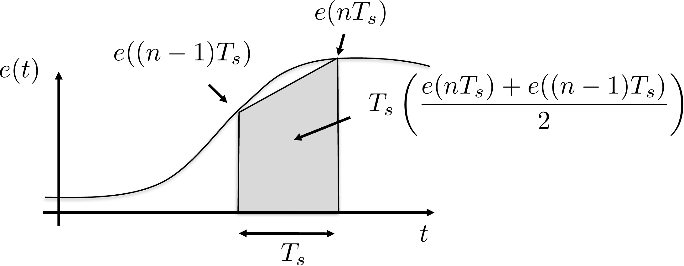
\end{aligned}\] As shown in
Fig.10.1, a trapezoidal
approximation of the integral between \((n-1)T_s\) and \(nT_s\) is given by \[\int_{(n-1)T_s}^{n T_s} e(\tau) d\tau \approx
\frac{T_s}{2}\left(e(nT_s)+e((n-1)T_s)\right).\]
Figure 10.1. Trapezoidal rule for digital
integration.
Therefore \[u_I(nT_s) \approx
u_I((n-1)T_s) + \frac{T_s}{2}\left(e(nT_s)+e((n-1)T_s)\right).\]
Taking the z-transform we get \[U_I(z) = z^{-1}U_I(z) +
\frac{T_s}{2}(E(z)+z^{-1}E(z)).\] Solving for \(U_I(z)\) gives \[\tag{10.1}
U_I(z) = \frac{T_s}{2}
\left(\frac{1+z^{-1}}{1-z^{-1}}\right)E(z).\] Since in the
Laplace domain we have \[U_I(s) =
\frac{1}{s}E(s),\] we have derived the so-called Tustin
approximation where \(s\) in the Laplace domain is replaced with
the \(z\)-transform approximation \[\tag{10.2}
s \mapsto \frac{2}{T_s}\left(\frac{1-z^{-1}}{1+z^{-1}}\right),\]
where \(T_s\) is the sample
period [18]. Taking the inverse
\(z\)-transform of
Equation 10.1 gives the discrete time
implementation of an integrator as \[\tag{10.3}
u_I[n] = u_I[n-1] + \frac{T_s}{2}\left(e[n] +
e[n-1]\right).\]
In the Laplace domain, a pure differentiator is given by \(U_D(s) = s E(s)\). However, since a pure
differentiator is not causal, the standard approach is to use the
band-limited, or dirty derivative \[U_D(s) =
\frac{s}{\sigma s + 1}E(s),\] where \(\sigma\) is small, and \(\frac{1}{\sigma}\) defines the bandwidth of
the differentiator. In practical terms, the dirty derivative differentiates signals
with frequency content less than \(\frac{1}{\sigma}\) radians per second.
Using the Tustin
approximation 10.2,
the dirty derivative in the \(z\)-domain becomes \[\begin{aligned}
U_D(z) &=
\frac{\frac{2}{T_s}\left(\frac{1-z^{-1}}{1+z^{-1}}\right)}{\frac{2\sigma}{T_s}\left(\frac{1-z^{-1}}{1+z^{-1}}\right)+1}E(z)
=
\frac{\left(\frac{2}{2\sigma+T_s}\right)(1-z^{-1})}{1-\left(\frac{2\sigma-T_s}{2\sigma+T_s}\right)z^{-1}}E(z).
\end{aligned}\] Transforming to the time domain, we have \[\tag{10.4}
u_D[n] = \left(\frac{2\sigma-T_s}{2\sigma+T_s}\right) u_D[n-1] +
\left(\frac{2}{2\sigma+T_s}\right)\left(e[n]-e[n-1]\right).\]
Interactive Figure 10.I1
Dirty derivative noise filtering
A pure finite-difference derivative reacts strongly to measurement
noise. The dirty derivative keeps the derivative causal and
band-limited; increasing sigma lowers the differentiator bandwidth and
smooths the derivative estimate.
Interactive Figure 10.I1. The upper plot
shows the noisy input signal v(t) and the true signal before measurement
noise is added. The lower plot compares the true derivative with the raw
finite-difference derivative and the dirty derivative. Use sigma to see
the tradeoff between noise rejection and lag.
A potential problem
with a straightforward implementation of PID controllers is integrator
windup. When the error \(r-y\) is large
and persists for an extended period, the value of the integrator can
become large, or “wind up.” A large integrator will cause \(u\) to saturate, which will cause the
system to push with maximum effort in the direction needed to correct
the error. Since the value of the integrator will continue to wind up
until the error signal changes sign, the control signal may not come out
of saturation until well after the error has changed sign, which can
cause a large overshoot and may destabilize the system.
Since integrator windup can destabilize the system, it is important
to add an anti-windup scheme. A number of different anti-windup schemes
are possible. In this section we will discuss two schemes that are
commonly used in practice. The first scheme is based on the fact that
integrators are typically used to correct for steady-state error and the
fact that overshoot is caused by integrating error during the transients
of the step response. Therefore, the integrator can be turned off when
the derivative of the error is large. This anti-windup scheme is
implemented by an if-statement conditioned on the size of
\(\dot{e}\).
The second anti-windup scheme is to subtract from the integrator
exactly the amount needed to keep \(u\)
at the saturation bound. In particular, let \[u_{\text{unsat}}=k_P e + k_D u_D + k_I
u_I\] denote the unsaturated control value before applying the
anti-windup scheme. After the saturation block we get \[u = \text{sat}(u_{\text{unsat}}) = \text{sat}(k_P
e + k_D u_D + k_I u_I).\] The idea of anti-windup is to modify
the output of the integrator from \(u_I\) to \(u_I^{+}\) so that \[k_P e + k_D u_D + k_I u_I^{+} = \text{sat}(k_P e
+ k_D u_D + k_I u_I) = u.\] Subtracting \(u_{\text{unsat}}\) from \(u\) gives \[\begin{aligned}
u-u_{\text{unsat}} &= (k_P e + k_D u_D + k_I u_I^{+})-(k_P e + k_D
u_D + k_I u_I) \\
&= k_I(u_I^{+}-u_I).
\end{aligned}\] Solving for \(u_I^{+}\) gives \[u_I^{+} = u_I +
\frac{1}{k_I}(u-u_{\text{unsat}}),\] which is the updated value
of the integrator that ensures that the control signal remains just out
of saturation. Note that if the control value is not in saturation then
\(u=u_{\text{unsat}}\) and the
integrator value remains unchanged.
Interactive Figure 10.I2
Anti-windup response under actuator saturation
Compare a saturated PI controller with and without anti-windup on an
intentionally underdamped second-order plant. The dashed traces show the
no-anti-windup baseline; the colored traces show the selected
controller. Use the actuator limit and integral gain to make windup more
or less severe.
Interactive
Figure 10.I2. The top plot shows the step response, the middle plot
shows uunsat and usat, and the bottom plot
shows the integrator state. Without anti-windup, the controller keeps
integrating error while the actuator is saturated, so
uunsat stays far beyond the actuator limit and the stored
integrator drives a large overshoot. The axes rescale so this growth
remains visible.
Overshoot
Time in saturation
Final error
Peak integrator
state
Interpretation: windup is visible when uunsat remains far
outside the actuator limit and the integrator state keeps growing.
Anti-windup changes the stored integrator state, so the controller
leaves saturation sooner and overshoots less.
10.1.2 Implementation
Python code that implements a general class for a PID loop is shown
below.
import numpy as npclass PIDControl:def__init__(self, kp, ki, kd, limit, sigma, Ts, flag=True):self.kp = kp # Proportional control gainself.ki = ki # Integral control gainself.kd = kd # Derivative control gainself.limit = limit # The output saturates at this limitself.sigma = sigma # dirty derivative bandwidth is 1/sigmaself.beta = (2.0*sigma-Ts)/(2.0*sigma+Ts)self.Ts = Ts # sample rateself.flag = flag# if flag == True, then returns# u = kp * error + ki * integral(error) + kd * error_dot.# else returns# u = kp * error + ki * integral(error) - kd * y_dot.self.y_dot =0.0# estimated derivative of yself.y_d1 =0.0# Signal y delayed by one sampleself.error_dot =0.0# estimated derivative of errorself.error_d1 =0.0# Error delayed by one sampleself.integrator =0.0# integratordef PID(self, r, y):# Compute the current error error = r - y# integrate error using trapazoidal ruleself.integrator =self.integrator + (self.Ts/2) * (error +self.error_d1)# PID Controlif flag isTrue:# differentiate errorself.error_dot =self.beta *self.error_dot + (1-self.beta)/self.Ts * (error -self.error_d1)# PID control u_unsat =self.kp*error +self.ki*self.integrator +self.kd*self.error_dotelse:# differentiate yself.y_dot =self.beta *self.y_dot + (1-self.beta)/self.Ts * (y -self.y_d1)# PID control u_unsat =self.kp*error +self.ki*self.integrator -self.kd*self.y_dot# return saturated control signal u_sat =self.saturate(u_unsat)# integrator anti - windupifself.ki !=0.0:self.integrator =self.integrator +self.Ts /self.ki * (u_sat - u_unsat)# update delayed variablesself.error_d1 = errorself.y_d1 = yreturn u_satdef PD(self, r, y):# Compute the current error error = r - y# PD Controlif flag isTrue:# differentiate errorself.error_dot =self.beta *self.error_dot + (1-self.beta)/self.Ts * (error -self.error_d1)# PD control u_unsat =self.kp*error +self.kd*self.error_dotelse:# differentiate yself.y_dot =self.beta *self.y_dot + (1-self.beta)/self.Ts * (y -self.y_d1)# PD control u_unsat =self.kp*error -self.kd*self.y_dot# return saturated control signal u_sat =self.saturate(u_unsat)# update delayed variablesself.error_d1 = errorself.y_d1 = yreturn u_satdef saturate(self,u):ifabs(u) >self.limit: u =self.limit*np.sign(u)return u
The PID controller class is initialized on lines 4–21, where
kp, ki, and kd are the control
gains, limit is the saturation limit for the control
signal, sigma is the dirty derivative gain, Ts
is the sample rate, and flag is a flag that indicates
whether the controller differentiates the error or the output. The
internal memory used to implement the differentiators and integrators is
initialized to zero in lines 17–21, where y_d1 is the
signal \(y\) delayed by one sample and
error_d1 is the error delayed by one sample. PID control is
implemented in lines 23–55 and PD control is implemented in lines 57–80.
The integrator update is shown in lines 50–51.
10.1.3 Gain Selection for PID
control
Gain selection for PID control usually proceeds in the following
manner. The proportional and derivative gains \(k_P\) and \(k_D\) are first selected according to the
methods discussed in
Chapter 11. The integral gain \(k_I\) is then tuned by starting with zero
and then slowly increasing the gain until the steady-state error is
removed. The parameters associated with the anti-windup scheme,
especially \(\bar{v}\), are also
adjusted during this phase. The proportional and derivative gains can
then be adjusted if necessary by retuning \(\omega_n\) and \(\zeta\). In the case of successive loop
closure, integrators are only
added on the outer loop.
The addition of an integrator has a destabilizing effect on the
feedback system. This effect is most easily understood by using the root
locus method described in
Appendix 30, where it can be seen that
for second-order systems, a large \(k_I\) will always result in closed-loop
poles in the right half-plane. The root locus can also be used to aid in
the selection of the integral gain \(k_I\), where the value of \(k_I\) is selected so that integrator has
minimal impact on the closed-loop poles designed using PD control. A
more effective method for selecting integral gains will be discussed in
Chapter 15.
The objective of this problem is to implement the PID controller
using only measured outputs of the system.
(a) Modify the system dynamics file so that the parameters vary by up to 20%
each time they are run (uncertainty parameter = 0.2).
(b) Change the simulation files so that the input to the controller is the
output and not the state. The controller should only assume knowledge of
the angle \(\theta\) and the reference
angle \(r_\theta\).
(c) Implement the PID controller designed in
Problems 3.1.11. Use the dirty derivative
gain of \(\sigma=0.05\). Tune the
integrator to remove the steady-state error caused by the uncertain
parameters.
Design Study A guided exercise
Assemble the digital PID controller
Identify the
implementation pieces that belong in the sampled controller class.
Step 1. Available feedback signal
Show solution for Step
1
Answer: The controller uses the
measured arm angle \(\theta\) and
the reference command.
Step 2. Discrete implementation choices
Show solution for
Step 2
Answer: Use trapezoidal
integration for the integral term and a dirty derivative for the
derivative term.
Step 3. Why simulate with uncertainty?
Show solution for
Step 3
Answer: The implementation
should be checked against parameter uncertainty and actuator limits, not
only the nominal continuous-time equations.
Pseudocode
The complete solution includes PID
implementation code. Before opening it, outline how you would update the
integrator, compute the dirty derivative, apply anti-windup, and return
the control torque.
This prompt is ungraded. It is intended to
connect the digital PID concepts to the implementation code in the
complete solution.
Complete solution
A Python class that implements a PID controller for the single link
robot arm is shown below.
The objective of this problem is to implement the PID controller
using only measured outputs of the system.
(a) Modify the system dynamics file so that the parameters \(m_1\), \(m_2\), \(\ell\) and \(b\) vary by up to 20% of their nominal
value each time they are run (uncertainty parameter = 0.2).
(b) Change the simulation files so that the input to the controller is the
output and not the state. The controller should only assume knowledge of
the position \(z\) and the angle \(\theta\), as well as the reference position
\(r_z\). Track a square wave with
amplitude of 0.5 meters and a frequency of 0.04 Hz.
(c) Implement the nested PID loops designed in
Problems 3.2.11. Use the dirty derivative
gain of \(\sigma=0.05\). Tune the
integrator to remove the steady-state error caused by the uncertain
parameters.
Design
Study B guided exercise
Prepare the nested digital PID
implementation
Identify measured signals, dirty derivatives,
uncertainty, and integral tuning.
Step 1. Available controller
inputs
Show solution for Step
1
Answer: The controller uses
measured z, measured theta, and the cart-position
reference.
Step 2. Derivative implementation
Show solution for Step
2
Answer: The implementation uses
dirty derivatives with sigma = 0.05.