This part of the book introduces the loop-shaping design method based on
the frequency response characteristics of the
system. In Part II we derived
transfer function and state-space models based on the linearized system.
In Part III we showed that PID controllers
can be used to regulate the output of second-order systems. For
higher-order systems, PID can be used if the original system can be
written as a cascade, or series, of second-order systems. In
Part IV we showed
that controllers can be derived for higher-order systems using
state-space models. The state-space design method is a time-domain
method that focuses on shaping the time-response of the system. In this
part of the book we extend PID control using frequency domain ideas
where we shape the frequency response of the system. When the transfer
function is available, it
provides a compact representation of the frequency response of the
open-loop system. Therefore, in this part we will focus on transfer
function models of the system. The methods in this part are not
constrained to second-order systems and do not depend on a cascade
structure. In fact, they do not even require a transfer function of the
system, as long as the frequency response, or Bode plot, is known.
Chapter 18 is a review of frequency
response models of linear time-invariant systems and develops intuition
concerning the Bode plot of the input-output response. In
Chapter 19 we show how
performance specifications for reference tracking, disturbance
rejection, and noise attenuation can be related to the frequency
response of the open loop control-plant pair.
Chapter 20 addresses stability of the
closed-loop system from a frequency response point of view.
Chapter 21 represents the
culminating chapter in this part of the book and describes how to design
the controller to achieve closed-loop stability and to satisfy design
specifications on reference tracking, disturbance rejection, and noise
attenuation.
15 Frequency Response of LTI
Systems
15.1 Theory
15.1.1 Manipulating Complex
Numbers
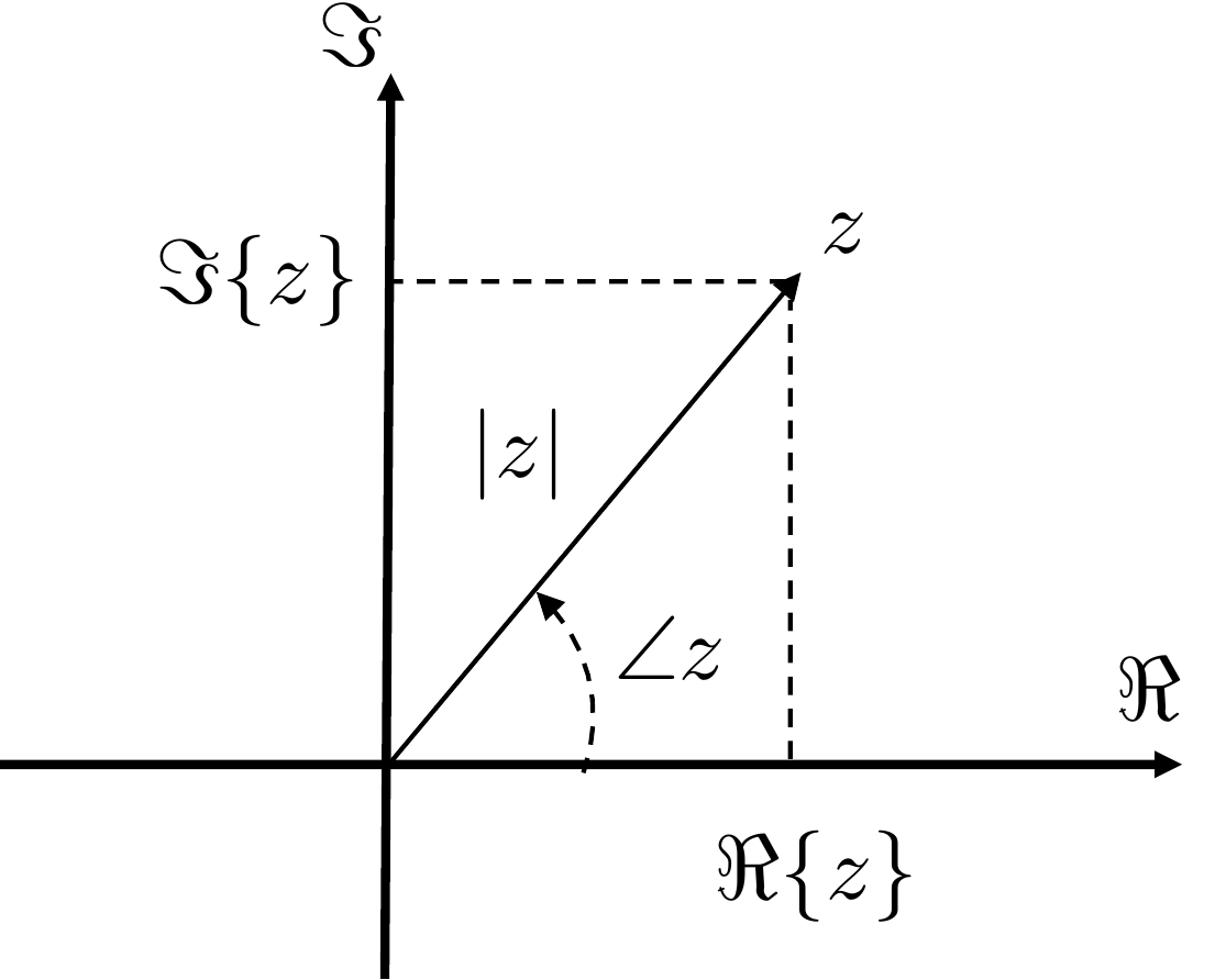
Any complex number \(z\) can be represented in rectangular
coordinates as \[z = \Re\{z\} + j \Im\{z\},\] where \(\Re\{z\}\) is the real part of \(z\), and \(\Im\{z\}\) is the imaginary part of \(z\). Similarly, \(z\) can be represented in polar
form as \[\tag{15.1}
z = \left|z\right|e^{j\angle z},\] where \(\left|z\right|\) denotes the magnitude of
\(z\) and \(\angle z\) denotes the angle or phase of
\(z\). The relationship
between the real and imaginary parts, and the magnitude and phase of
\(z\), are depicted in
Fig.15.1.
Figure 15.1. Relationship between the real and
imaginary parts of z, and the
magnitude and phase of z.
From the geometry shown in
Fig.15.1 we can see that \[\begin{aligned}
\left|z\right| &= \sqrt{\Re\{z\}^2 + \Im\{z\}^2} \\
\angle z &= \tan^{-1}\frac{\Im\{z\}}{\Re\{z\}}.
\end{aligned}\] Similarly, from Euler’s relationship \[e^{j\theta} = \cos\theta + j\sin\theta,\]
we have from
Equation 15.1 that \[z = \left|z\right|e^{j\angle z} =
\left|z\right|\cos\angle z + j \left|z\right|\sin\angle z\] which
implies that \[\begin{aligned}
\Re\{z\} &= \left|z\right|\cos\angle z \\
\Im\{z\} &= \left|z\right|\sin\angle z.
\end{aligned}\]
The conjugate of \(z\), denoted
\(\bar{z}\), is given by \[\bar{z} = \Re\{z\}-j\Im\{z\} =
\left|z\right|e^{-j\angle z}.\] Note that \(z\bar{z} = \left|z\right|^2\).
Suppose that \(z_1 =
\left|z_1\right|e^{j\angle z_1}\) and \(z_2=\left|z_2\right|e^{j\angle z_2}\) are
two complex numbers, then \[\begin{aligned}
z_1z_2 &= \left|z_1\right|e^{j\angle z_1}\left|z_2\right|e^{j\angle
z_2} \\
&= \left|z_1\right|\left|z_2\right|e^{j\angle z_1}e^{j\angle
z_2} \\
&= \left|z_1\right|\left|z_2\right|e^{j(\angle z_1 + \angle
z_2)},
\end{aligned}\] therefore when multiplying complex numbers, their
magnitudes multiply, but their phases add. Similarly, we have \[\frac{z_1}{z_2} =
\frac{\left|z_1\right|e^{j\angle z_1}}{\left|z_2\right|e^{j\angle z_2}}
= \frac{\left|z_1\right|}{\left|z_2\right|}\frac{e^{j\angle
z_1}}{e^{j\angle z_2}}
= \frac{\left|z_1\right|}{\left|z_2\right|}e^{j(\angle z_1 -
\angle z_2)},\] therefore when dividing complex numbers, their
magnitudes divide, but their phases subtract.
A transfer function \(H(s)\) is a complex number for any specific
value of \(s\). Therefore, \(H(s)\) can be expressed in both rectangular
and polar forms as \[H(s) = \Re\{H(s)\} +
j\Im\{H(s)\} = \left|H(s)\right|e^{j\angle H(s)}.\] For example,
if \(H(s) = \frac{1}{s+1}\), then when
\(s=2+j3\)\[\begin{aligned}
H(2+j3) &= \frac{1}{2+j3+1}= \frac{1}{3+j3} =
\frac{1}{3+j3}\frac{3-j3}{3-j3} \\&= \frac{1}{6} - j\frac{1}{6} =
\sqrt{\frac{1}{18}}e^{-j\frac{\pi}{4}}.
\end{aligned}\] If \(H(s)\) has
multiple poles and zeros, then the magnitude and phase of \(H(s)\) can be represented in terms of the
magnitude and phase of the poles and zeros. For example, suppose that
\[H(s) =
\frac{K(s+z_1)(s+z_2)\dots(s+z_m)}{(s+p_1)(s+p_2)\dots(s+p_n)}.\]
Since \((s+a)\) is a complex number for
any \(s\), it can be written in polar
form as \(s+a=\left|s+a\right|e^{j\angle(s+a)}\),
therefore \[\begin{aligned}
H(s) &=
\frac{K(s+z_1)(s+z_2)\dots(s+z_m)}{(s+p_1)(s+p_2)\dots(s+p_n)} \\
&= \frac{\left|K\right|e^{j\angle K}
\left|s+z_1\right|e^{j\angle(s+z_1)}\left|s+z_2\right|e^{j\angle(s+z_2)}\dots\left|s+z_m\right|e^{j\angle(s+z_m)}}
{\left|s+p_1\right|e^{j\angle(s+p_1)}\left|s+p_2\right|e^{j\angle(s+p_2)}\dots\left|s+p_n\right|e^{j\angle(s+p_n)}}
\\
&=
\frac{\left|K\right|\left|s+z_1\right|\left|s+z_2\right|\dots\left|s+z_m\right|}{\left|s+p_1\right|\left|s+p_2\right|\dots\left|s+p_n\right|}
\frac{e^{j\angle K} e^{j\angle(s+z_1)}e^{j\angle(s+z_2)}\dots
e^{j\angle(s+z_m)}}{e^{j\angle(s+p_1)}e^{j\angle(s+p_2)}\dots
e^{j\angle(s+p_n)}} \\
&=
\frac{\left|K\right|\left|s+z_1\right|\left|s+z_2\right|\dots\left|s+z_m\right|}{\left|s+p_1\right|\left|s+p_2\right|\dots\left|s+p_n\right|}
e^{j\left(\angle K + \sum_{i=1}^m \angle (s+z_i) - \sum_{i=1}^n
\angle (s+p_i)\right)}.
\end{aligned}\] Therefore \begin{align}
\left|H(s)\right| &=
\frac{\left|K\right|\left|s+z_1\right|\left|s+z_2\right|\dots\left|s+z_m\right|}{\left|s+p_1\right|\left|s+p_2\right|\dots\left|s+p_n\right|}
\tag{15.2}\\
\angle H(s) &= \angle K + \sum_{i=1}^m \angle (s+z_i) - \sum_{i=1}^n
\angle (s+p_i). \tag{15.3}
\end{align}
15.1.2 Frequency Response of LTI
Systems
In systems theory, the magnitude and phase representations of the
transfer function \(H(s)\) are used
because they have important physical meaning. In particular, suppose
that \(H(s)\) represents a physical
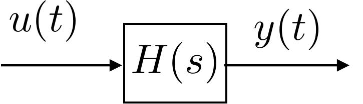
system with input \(u(t)\) and output
\(y(t)\) as shown in
Fig.15.2.
Figure 15.2. LTI system represented by the transfer
function H(s) with
input u(t) and output
y(t).
If the input to the system is given by a sinusoid of magnitude \(A\) and frequency \(\omega_0\), i.e., \[u(t) = A\sin(\omega_0t),\] then the output
is given by \[\tag{15.4}
y(t) = A\left|H(j\omega_0)\right|\sin(\omega_0 t + \angle
H(j\omega_0)).\] Therefore, the transfer function \(H(s)\) is an elegant and compact
representation of the frequency response of the system, in that the
magnitude of \(H(j\omega_0)\) describes
the gain of the system for input signals with frequency \(\omega_0\), and the phase of \(H(j\omega_0)\) describes the phase shift
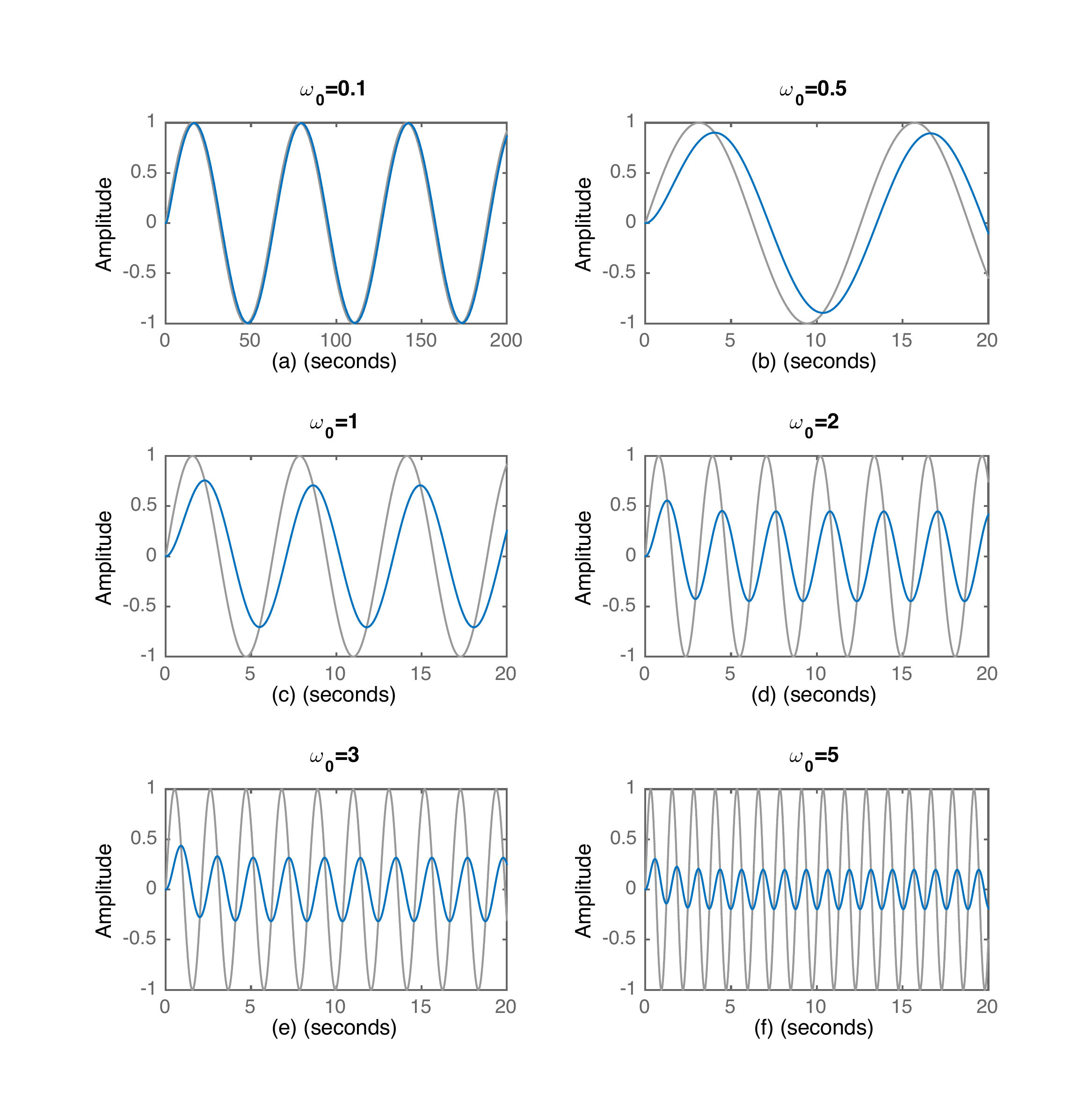
imposed by the system on input signals with frequency \(\omega_0\). For example,
Fig.15.3 shows the input-output
response of an LTI system with transfer function \(H(s)=\frac{1}{s+1}\). The input signal,
which is shown in grey, is \(u(t)=\sin(\omega_0 t)\) where \(\omega_0\) changes in each subplot. The
output signal is shown in blue and is given by
Equation 15.4. Note
that in subplot (a) the time scale is different from that of the other
subplots. When \(\omega_0=0.1\), \(H(j\omega_0)\approx 0.995e^{j5^\circ}\).
Accordingly, in subplot (a), the output is only slightly attenuated,
with very little phase shift. In contrast, when \(\omega_0=5\), \(H(j\omega_0)\approx 0.2 e^{j80^\circ}\),
and in subplot (f) we see that the output is approximately 20% of the
input with a phase shift approaching \(90\) degrees.
Figure 15.3. Frequency response to LTI system with
transfer function H(s) = 1/(s + 1).
Chapter 15 interactive figure
Sinusoidal input and steady-state output
For H(s)=1/(s+1), move the
input frequency. The output amplitude and phase shift are computed from
H(jω), then plotted against the
input signal.
Interactive Figure 15.I1. Move the input
frequency to see how H(jw) changes the output amplitude and phase.
|H(jω)|
Phase shift
Interpretation
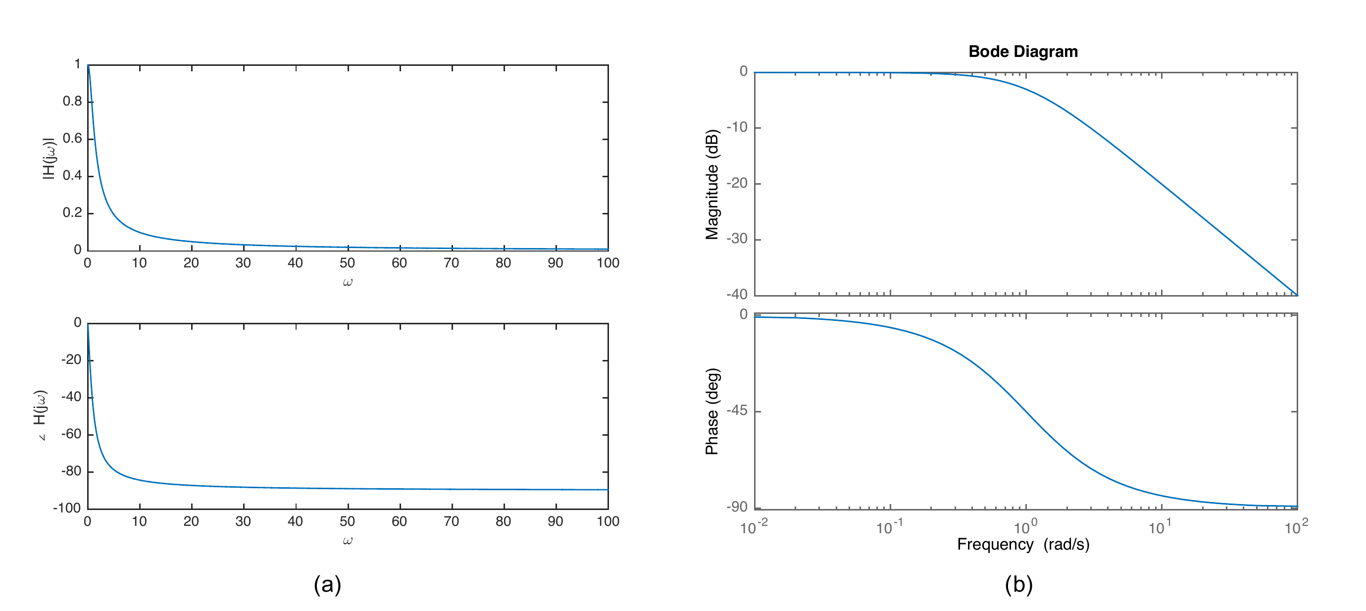
Therefore, the response of an LTI system to inputs at different
frequencies can be visualized by plotting the magnitude and phase of
\(H(j\omega)\) as a function of \(\omega\). The frequency response of \(H(s)=1/(s+1)\) is plotted in two different
ways in
Fig.15.4. In subfigure (a) a
linear scale is used for both \(\left|H(j\omega)\right|\) and \(\angle H(j\omega)\), as well as the
frequency scale \(\omega\). In
subfigure (b), the scale for magnitude is in dB: \(20\log\left|H(j\omega)\right|\) whereas the
scale for \(\angle H(j\omega)\) is
linear, however, in both cases a log scale for \(\omega\) is used on the \(x\)-axis. The plot in subfigure (b) is
called a Bode plot. It should be clear from
Fig.15.4 that the Bode plot
provides much more useful information than a linear plot since it more
effectively reveals the behavior of the system at lower frequencies. For
this reason, Bode plots are the most common method to display the
frequency response of the system.
Figure 15.4. Frequency response of H(s) = 1/(s + 1)
on a linear scale (a), and a logarithmic scale (b).
Chapter 15 interactive figure
Linear scale versus Bode scale
For H(s)=1/(s+1), move the
frequency marker. The left plot uses linear magnitude and linear
frequency; the right plot shows the same response as a Bode plot with dB
magnitude and log frequency.
Interactive
Figure 15.I2. Compare the same frequency response on a linear plot and
on a Bode plot. The shaded area on the linear plot shows how
low-frequency behavior is compressed when many decades are shown on a
linear axis.
Selected frequency
|H(jω)|
20log10|H(jω)|
∠H(jω)
Interpretation
dB conversion
reference:0 dB → |H| = 1-3 dB → |H| ≈ 0.707-20 dB → |H| = 0.1-40 dB → |H| = 0.01
Check your interpretation
Why is
the Bode plot more useful here?
As a note, since the magnitude of \(H(j\omega)\) is displayed on the Bode plot
as \(20\log\left|H(j\omega)\right|\) in
units of dB, note that \(20\log\left|H(j\omega)\right|=0\) dB
implies that \(\left|H(j\omega)\right|=1\). Similarly,
\(20\log\left|H(j\omega)\right|=20\) dB
implies that \(\left|H(j\omega)\right|=10\) and \(20\log\left|H(j\omega)\right|=40\) dB
implies that \(\left|H(j\omega)\right|=100\). Going in the
other direction, \(20\log\left|H(j\omega)\right|=-20\) dB
implies that \(\left|H(j\omega)\right|=0.1\), and \(20\log\left|H(j\omega)\right|=-40\) dB
implies that \(\left|H(j\omega)\right|=0.01\). In general,
\[20\log\left|H(j\omega)\right|=20n\text{~dB~}
\implies \left|H(j\omega)\right|=10^n.\]
15.1.3 Straight-line Approximations
for Bode Plots
While the Bode plot for a system can be easily generated using the
MATLAB or Python bode command, it is still useful to
understand how to approximately draw a Bode plot by hand. The reason for
this is that in the loop-shaping design methodology, we add elements to
the control transfer function \(C(s)\)
to "shape" the Bode plot of the loop gain \(P(s)C(s)\) where \(P(s)\) is the transfer function of the
plant. Learning to approximately draw the Bode plot by hand will provide
helpful insights into this process. Therefore, in this section we
provide a brief tutorial on how to approximate the Bode plot for a
transfer function \(H(s)\).
We start by putting the transfer function into Bode canonical
form by factoring out the poles and zeros as follows: \[\begin{aligned}
H(s) &=
\frac{K(s+z_1)(s+z_2)\dots(s+z_m)}{(s+p_1)(s+p_2)\dots(s+p_n)} \\
&= \frac{Kz_1z_2\dots z_m}{p_1p_2\dots
p_n}\frac{(1+s/z_1)(1+s/z_2)\dots(1+s/z_m)}{(1+s/p_1)(1+s/p_2)\dots(1+s/p_n)}.
\end{aligned}\] Therefore, following
Equations 15.2 and
15.3 we have \begin{align}
\left|H(j\omega)\right| &= \left|\frac{Kz_1z_2\dots z_m}{p_1p_2\dots
p_m}\right|
\frac{\left|1+j\omega/z_1\right|\left|1+j\omega/z_2\right|\dots\left|1+j\omega/z_m\right|}{\left|1+j\omega/p_1\right|\left|1+j\omega/p_2\right|\dots\left|1+j\omega/p_n)\right|}
\tag{15.5}\\
\angle H(j\omega) &= \angle \left(\frac{Kz_1z_2\dots
z_m}{p_1p_2\dots p_m}\right) + \sum_{i=1}^m \angle (1+j\omega/z_i) -
\sum_{i=1}^n \angle (1+j\omega/p_i). \tag{15.6}
\end{align} Since \(20\log\left|AB\right|=20\log\left|A\right|+20\log\left|B\right|\),
Equation 15.5 gives \begin{gather}
\tag{15.7}
20\log\left|H(j\omega)\right| = 20\log \left|\frac{Kz_1z_2\dots
z_m}{p_1p_2\dots p_m}\right| \\
+ \sum_{i=1}^m 20\log\left|1+j\omega/z_i\right| - \sum_{i=1}^n
20\log\left|1+j\omega/p_i\right|.
\end{gather}
Drawing the Bode plot for a general transfer function with real poles
and zeros, can be decomposed into drawing the Bode plot for each pole
and zero, and then graphically adding them to get the general Bode plot.
Note first that \[20\log
\left|\frac{Kz_1z_2\dots z_m}{p_1p_2\dots p_m}\right|\] is not a
function of \(\omega\) and is therefore
a constant line on the Bode plot. Also note that \[\angle \left(\frac{Kz_1z_2\dots z_m}{p_1p_2\dots
p_m}\right)\] is also a constant and is either \(0\) degrees if \(\left(\frac{Kz_1z_2\dots z_m}{p_1p_2\dots
p_m}\right)>0\), or \(180\) degrees if \(\left(\frac{Kz_1z_2\dots z_m}{p_1p_2\dots
p_m}\right)<0\).
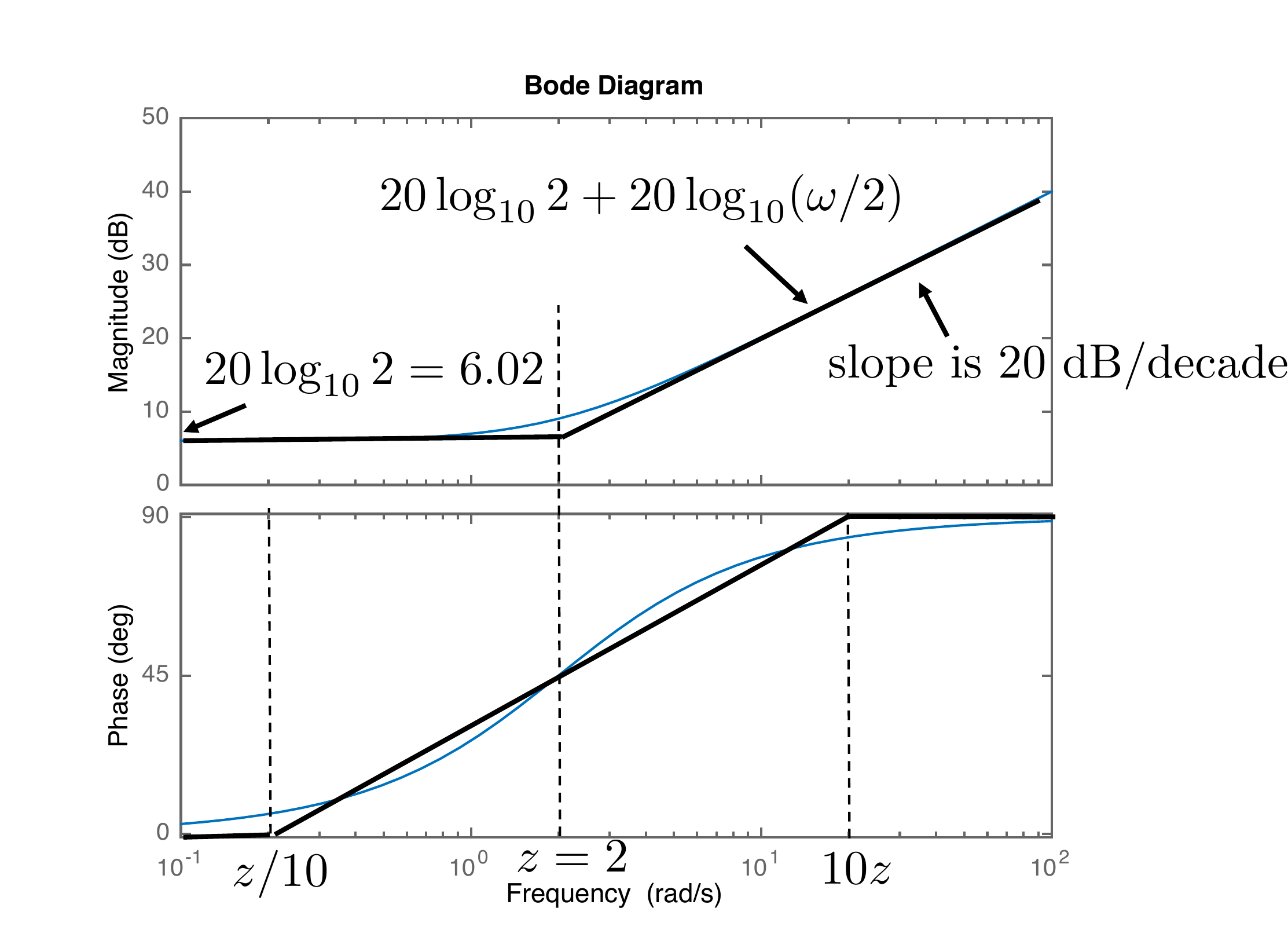
We start by drawing the Bode plot when \(H(s) = s+z\) has a single zero at \(s=-z\) and \(z>0\). The first step is to put the
transfer function in Bode canonical form as \[H(j\omega) = z(1+j\frac{\omega}{z}).\]
Therefore, from
Equation 15.7 we have \[\begin{aligned}
20\log\left|H(j\omega)\right| &= 20\log\left|z\right| +
20\log\left|1+j\frac{\omega}{z}\right| \\&= 20\log\left|z\right| +
20\log\sqrt{1+(\omega/z)^2}.
\end{aligned}\] When \(\omega/z\ll
1\) we have that \(\sqrt{1+(\omega/z)^2}\approx 1\), implying
that \[20\log\left|H(j\omega)\right| \approx
20\log\left|z\right|.\] Note that since this term is not a
function of \(\omega\), it is a
constant value on the Bode plot. On the other hand, when \(\omega/z \gg 1\) we have that \(\sqrt{1+(\omega/z)^2}\approx
\left|\omega/z\right|\), giving \[20\log\left|H(j\omega)\right| \approx
20\log\left|z\right| + 20\log\left|\omega/z\right|.\] Note that
the second term is a straight line on a Bode plot that intersects the
\(0\) dB axis at \(\omega=z\) and increases \(20\) dB for every factor of 10 increase in
\(\omega\). Therefore, on the Bode
plot, the slope of the second term is \(+20\) dB/decade. A straight-line
approximation is shown in
Fig.15.5, along with the Bode
plot produced by MATLAB.
Figure 15.5. Straight-line approximation for a single
zero.
Note that the largest mismatch between the straight-line
approximation and the actual Bode plot is at \(\omega=z\). In that case we have \[20\log\left|H(jz)\right| \approx
20\log\left|z\right| + 20\log\sqrt{2}=20\log\left|z\right| +
3~dB.\] Therefore, at the corner frequency \(z\) the Bode plot is \(3\) dB above the low frequency
response.
To approximate the phase plot, note that \[\tag{15.8}
\angle H(j\omega) = \angle z(1+j\omega/z)
=\tan^{-1}\frac{\omega}{z}.\] When \(\omega=z\) we have that \(\tan^{-1} 1 = 45\) degrees. When \(\omega\ll z\), we have that \(\tan^{-1}(\omega/z)\approx 0\) degrees, and
when \(\omega\gg z\), we have that
\(\tan^{-1}(\omega/z)\approx
90\) degrees. The phase plot as calculated by MATLAB is shown in
Fig.15.5. An adequate
straight-line approximation is obtained by setting the phase to zero
when \(\omega<z/10\), i.e., one
decade less than \(z\), and setting the
phase to \(90\) degrees when \(\omega>10z\), i.e., one decade greater
than \(z\), and drawing a straight line
between those points so that the phase at \(z\) is \(45\) degrees. The straight-line
approximation for the phase is also shown in black
in Fig.15.5.
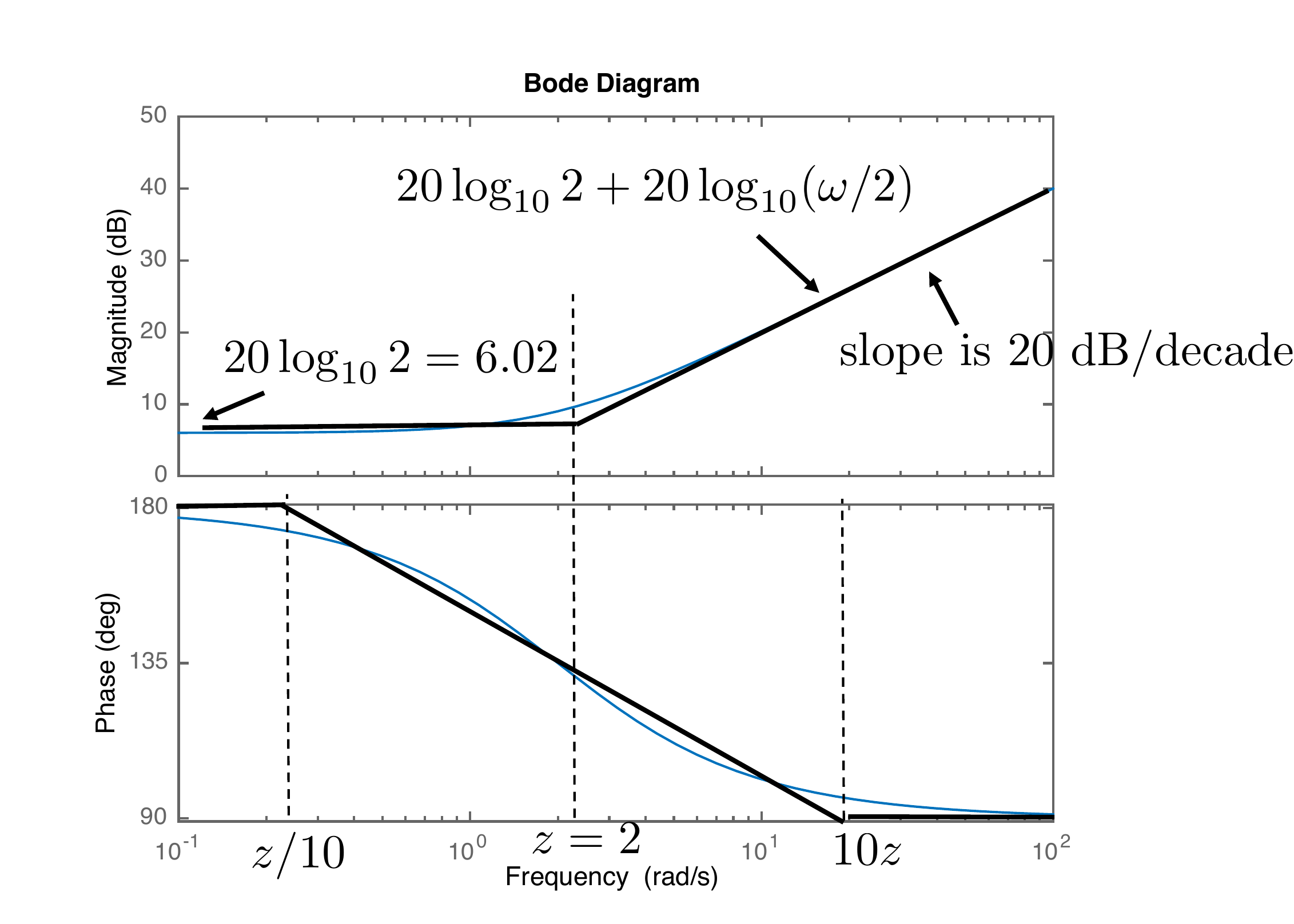
The straight-line approximation for phase as described above assumes
that \(z>0\), i.e., that the zero is
in the left half of the complex plane. For right-half-plane zeros when
\(z<0\), the phase as calculated in
Equation 15.6 is \[\angle H(j\omega) = \angle z + \angle
(1+j\omega/z) = 180^\circ -
\tan^{-1}\frac{\omega}{\left|z\right|}.\] Therefore, the phase
starts at \(180\) degrees and decreases
by \(90\) degrees as \(\omega\) gets large rather than increases.
Fig.15.6 shows the Bode
plot and its straight-line approximation when the zero is in the right
half-plane. When a system has a zero in the right half-plane, it is
called non-minimum phase because of the \(180\) degree phase increase at low
frequencies.
Figure 15.6. Straight-line approximation for a zero in
the right half of the complex plane.
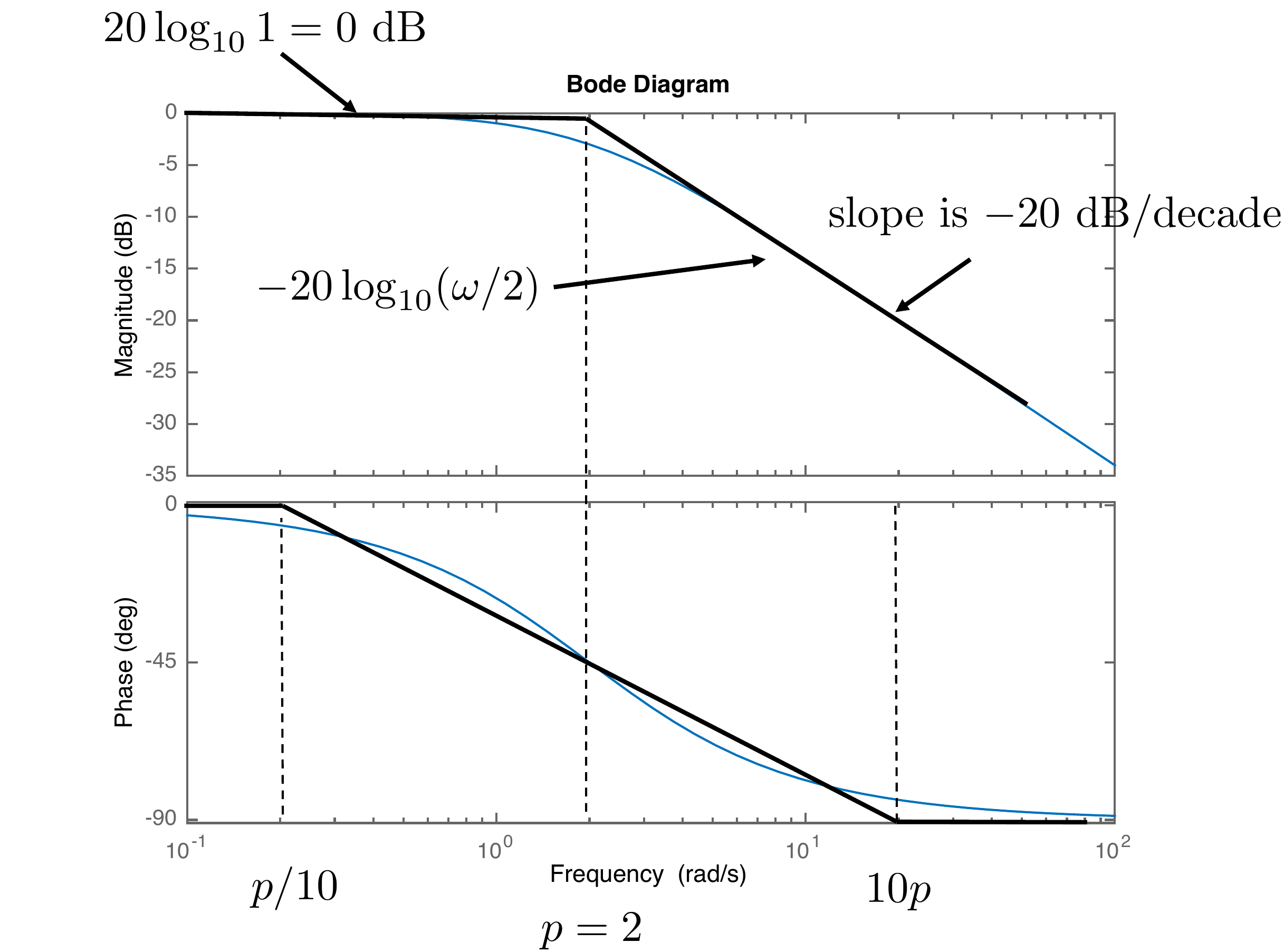
Now consider drawing the Bode plot for a single pole, i.e., \(H(s) = \frac{p}{s+p}\), which has a single
pole at \(s=-p\) which is in the right
half-plane when \(p>0\). In Bode
canonical form \(H(s)\) becomes \[H(j\omega) =
\frac{1}{1+j\frac{\omega}{p}}.\] Therefore, from
Equation 15.7 we have \[\begin{aligned}
20\log\left|H(j\omega)\right| &= 20\log\left|1\right| -
20\log\left|1+j\frac{\omega}{p}\right| \\&= -
20\log\sqrt{1+(\omega/p)^2}.
\end{aligned}\] When \(\omega/p\ll
1\), we have that \(\sqrt{1+(\omega/p)^2}\approx 1\), implying
that \[20\log\left|H(j\omega)\right| \approx
0.\] Note that since this term is not a function of \(\omega\), it is a constant value at \(0\) dB on the Bode plot. On the other hand,
when \(\omega/p \gg 1\), we have that
\(\sqrt{1+(\omega/p)^2}\approx
\left|\omega/p\right|\), giving \[20\log\left|H(j\omega)\right| \approx
-20\log\left|\omega/p\right|.\] Note that the second term is a
straight line on a Bode plot that intersects the \(0\) dB axis when \(\omega=p\) and decreases at \(-20\) dB for every factor of 10 increase in
\(\omega\). Therefore, on the Bode
plot, the slope of the second term is \(-20\) dB/decade. A straight-line
approximation is shown in
Fig.15.7, along with the Bode
plot produced by MATLAB.
Figure 15.7. Straight-line approximation for a single
pole.
Note that the largest mismatch between the straight-line
approximation and the actual Bode is at \(\omega=p\). In that case, we have \[20\log\left|H(jp)\right| \approx
-20\log\sqrt{2}=-3~dB.\] Therefore, at the corner frequency \(p\) the Bode plot is \(3\) dB below the low frequency
response.
To approximate the phase plot, note that \[\tag{15.9}
\angle H(j\omega) = -\angle (1+j\frac{\omega}{p}) =
-\tan^{-1}\frac{\omega}{p}.\] When \(\omega=p\) we have that \(-\tan^{-1} 1 = -45\) degrees. When \(\omega\ll p\), we have that \(-\tan^{-1}(\omega/p)\approx 0\) degrees,
and when \(\omega\gg p\), \(-\tan^{-1}(\omega/p)\approx -90\) degrees.
The phase plot as calculated by MATLAB is shown in
Fig.15.7. An adequate
straight-line approximation is obtained by setting the phase to zero
when \(\omega<p/10\), i.e., one
decade less than \(p\), and setting the
phase to \(-90\) degrees when \(\omega>10p\), i.e., one decade greater
than \(p\), and drawing a straight line
between those points so that the phase at \(p\) is \(-45\) degrees. The straight-line
approximation for the phase is also shown in
Fig.15.7.
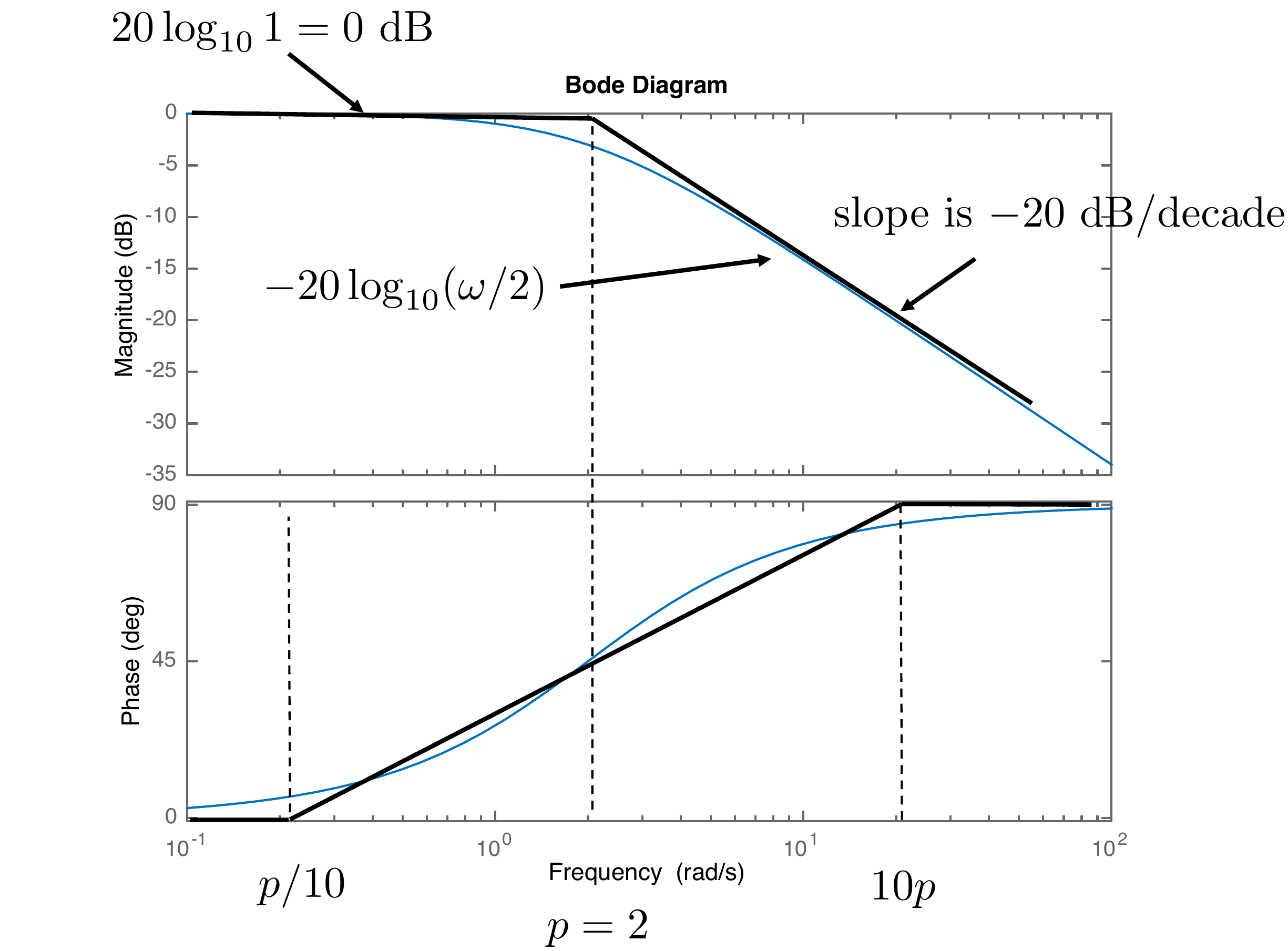
The straight-line approximation for phase as described above assumes
that \(p>0\), i.e., that the pole is
in the left half of the complex plane. For right-half-plane poles when
\(p<0\), the phase as calculated in
Equation 15.6 is \[\angle H(j\omega) = -\angle (1+j\omega/p) =
\tan^{-1}\frac{\omega}{\left|p\right|}.\] Therefore, the phase
starts at \(0\) degrees and increases
by \(90\) degrees as \(\omega\) gets large.
Fig.15.8 shows the Bode
plot and its straight-line approximation when the pole is in the right
half-plane. Note that stability and instability are not directly evident
from the shapes of the magnitude and phase plots.
Figure 15.8. Straight-line approximation for a pole in
the right half of the complex plane.
Chapter 15 interactive figure
Single pole/zero Bode builder
Choose one first-order factor and move the corner frequency. The plot
compares the exact Bode response with the straight-line approximation
used for hand sketches.
Interactive
Figure 15.I3. Compare exact first-order magnitude and phase with their
straight-line approximations.
Magnitude slope
Phase change
Corner value
Guide frequencies
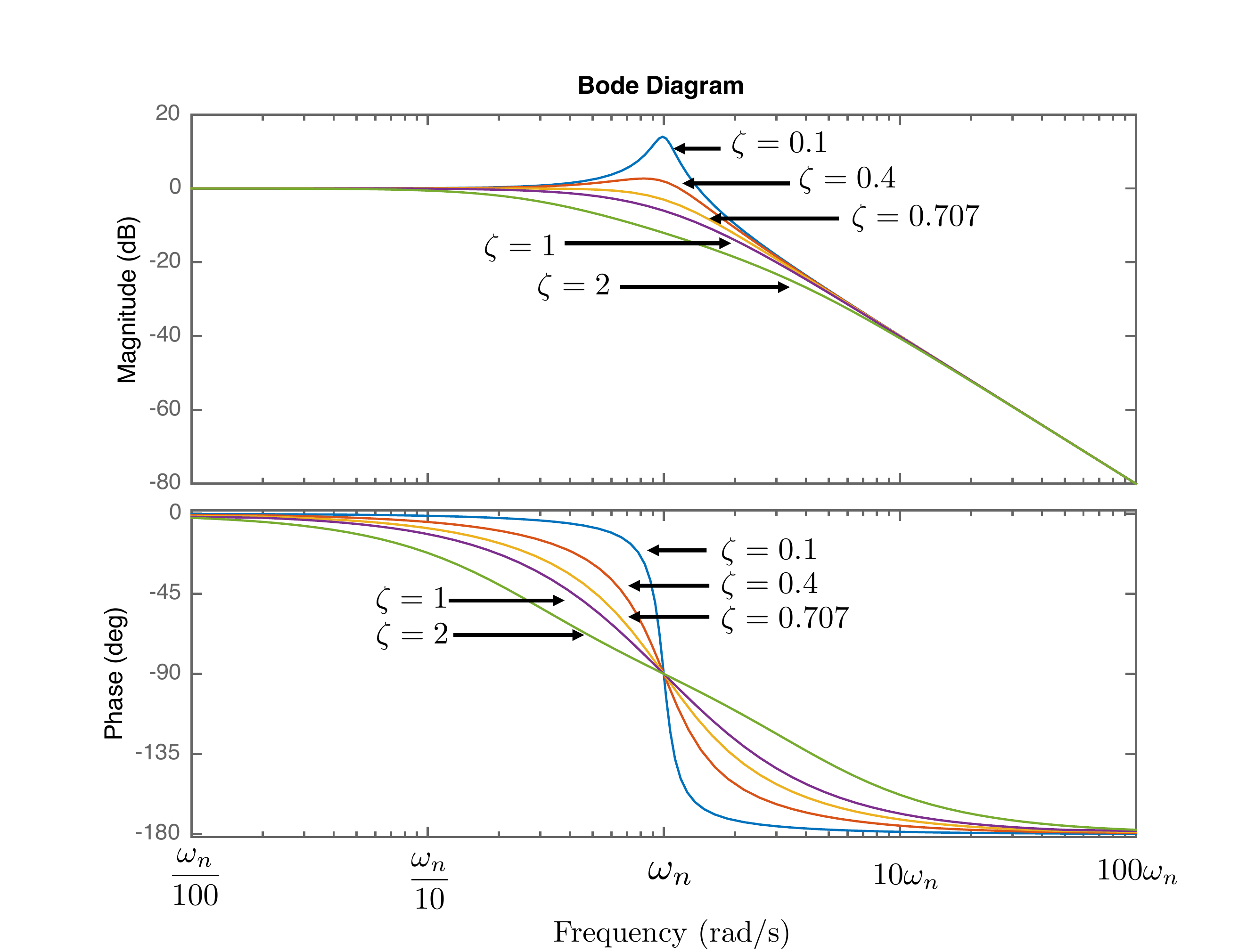
Suppose now that the poles are complex. Let \[H(s)=\frac{\omega_n^2}{s^2+2\zeta\omega_ns+\omega_n^2}.\]
In Bode canonical form we have \[\begin{aligned}
H(j\omega) &=
\frac{1}{\omega_n^2}\frac{\omega_n^2}{\frac{(j\omega)^2}{\omega_n^2} +
2\zeta\omega_n\left(\frac{j\omega}{\omega_n^2}\right) + 1}\\
&=
\frac{1}{\left(1-\left(\frac{\omega}{\omega_n}\right)^2\right) + j
2\zeta\left(\frac{\omega}{\omega_n}\right)} \\
&=
\frac{1}{\sqrt{\left(1-\frac{\omega^2}{\omega_n^2}\right)^2 +
4\zeta^2\frac{\omega^2}{\omega_n^2}}}
e^{-j\tan^{-1}\left(\frac{2\zeta\frac{\omega}{\omega_n}}{1-\frac{\omega^2}{\omega_n^2}}\right)}.
\end{aligned}\] Therefore \[\begin{aligned}
\left|H(j\omega)\right| &=
\frac{1}{\sqrt{\left(1-\frac{\omega^2}{\omega_n^2}\right)^2 +
4\zeta^2\frac{\omega^2}{\omega_n^2}}} \\
\angle H(j\omega) &=
-\tan^{-1}\left(\frac{2\zeta\frac{\omega}{\omega_n}}{1-\frac{\omega^2}{\omega_n^2}}\right).
\end{aligned}\] When \(\omega \ll
\omega_n\) we have that \(20\log_{10}\left|H(j\omega)\right|\approx
20\log_{10}\left|1\right| = 0\) dB. Also, \(\angle H(j\omega)\approx
-\tan^{-1}\frac{0}{1}=0\) degrees. Alternatively, when \(\omega \gg \omega_n\) we have \[\begin{aligned}
20\log_{10}\left|H(j\omega)\right| &\approx -20\log
\sqrt{\left(\frac{\omega^2}{\omega_n^2}\right)^2 +
4\zeta^2\frac{\omega^2}{\omega_n^2}} \\
&\approx -20\log
\sqrt{\left(\frac{\omega^2}{\omega_n^2}\right)^2} \\
&\approx -20\log
\left|\frac{\omega}{\omega_n}\right|^2 \\
&= -40\log
\left|\frac{\omega}{\omega_n}\right|,
\end{aligned}\] which is a straight line that crosses the \(0\) dB axis at \(\omega_n\) with a slope of \(-40\) dB/decade. When \(\omega=\omega_n\) we have \(20\log_{10}\left|H(j\omega)\right| =
-20\log_{10}\sqrt{4\zeta^2} = -20\log_{10}\left|2\zeta\right|\).
When \(\zeta=0.707=\frac{\sqrt{2}}{2}\), then
\(20\log_{10}\left|H(j\omega)\right|=-20\log_{10}1/\sqrt{2}
=-3\) dB. For the angle plot, when \(\omega \ll \omega_n\) we have \(\angle H(j\omega)\approx \tan^{-1}\frac{0}{1} =
0\) degrees. When \(\omega \gg
\omega_n\) we have \(\angle H(j\omega)
\approx \tan^{-1}\left(2\zeta \frac{\omega_n}{\omega}\right)\approx
-180\) degrees, and when \(\omega=\omega_n\) we have \(\angle H(j\omega)\approx -
\tan^{-1}\frac{2\zeta}{0}=-90\) degrees.
The Bode plots for different values of \(\zeta\) are shown in
Fig.15.9.
Figure 15.9. The Bode plot for a second-order system
for various values of ζ.
Chapter 15 interactive figure
Second-Order System Bode response
Move the damping ratio and natural frequency for
H(s) = ωn2 /
(s2 + 2ζωns + ωn2).
Low damping creates resonant peaking near
ωn.
Interactive Figure 15.I4. Move ζ and ωn to see
resonant peaking, phase transition, and -40 dB/dec high-frequency
rolloff.
Peak magnitude
Phase at ωn
High-frequency
slope
15.1.4 Example
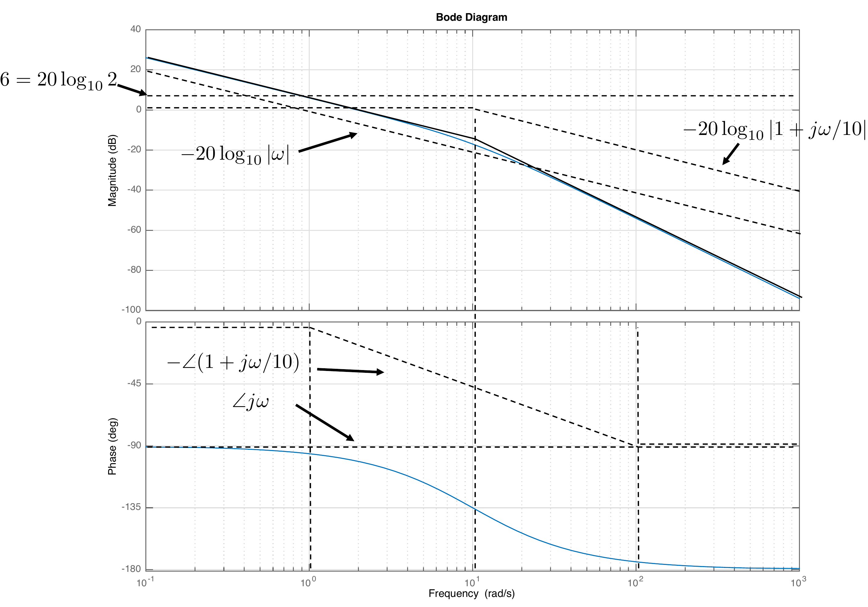
Find the straight-line approximation for the Bode plot of the
transfer function \[\tag{15.10}
H(s) = \frac{20}{s(s+10)}.\] In Bode canonical form we have \[H(j\omega) =
\frac{20}{10}\frac{1}{j\omega(1+j\frac{\omega}{10})}.\] Therefore
\begin{gather}
\tag{15.11}
20\log_{10}\left|H(j\omega)\right|= \\ 20\log_{10} 2 -
20\log_{10}\left|\omega\right| -
20\log_{10}\sqrt{1+\left(\frac{\omega}{10}\right)^2}.
\end{gather} Note that the term due to the pole at zero,
namely \(-20\log_{10}\left|\omega\right|\) is a
straight line that intercepts the \(0\) dB line at \(\omega=1\), and has a slope of \(-20\) dB per decade. Therefore, the Bode
plot for magnitude will be the graphical addition of three terms:
A constant term at \(20\log_{10} 2 =
2\) dB,
A straight line with slope of \(-20\) dB/decade, passing through the \(0\) dB line at \(\omega=1\), and
A first order low-pass filter with a cut-off frequency at \(\omega=10\).
Similarly, the phase is given by \[\begin{aligned}
\angle H(j\omega) &= \angle 2 - \angle j\omega - \angle
(1+j\frac{\omega}{10}) \\
&= 0 - \tan^{-1}\frac{\omega}{0} -
\tan^{-1}\frac{\omega}{10} \\
&= - 90^\circ -
\tan^{-1}\frac{\omega}{10}.
\end{aligned}\] The straight-line approximation and the Bode plot
generated by MATLAB are shown in
Fig.15.10.
Figure 15.10. Bode plot for the transfer function given
in Equation 15.10.
Chapter 15 interactive figure
Build Example 15.1.4 term by term
Turn on each factor in H(s) = 20/(s(s+10)) to see how the straight-line
magnitude and phase approximations are built by graphical addition. The
exact full response stays visible as a reference.
Interactive
Figure 15.I5. The gray curves show active individual terms, the black
dashed curve shows their cumulative straight-line approximation, and the
colored curve shows the exact full response.
Active terms
Current lesson
Probe magnitude
Probe phase
15.1.5 Example
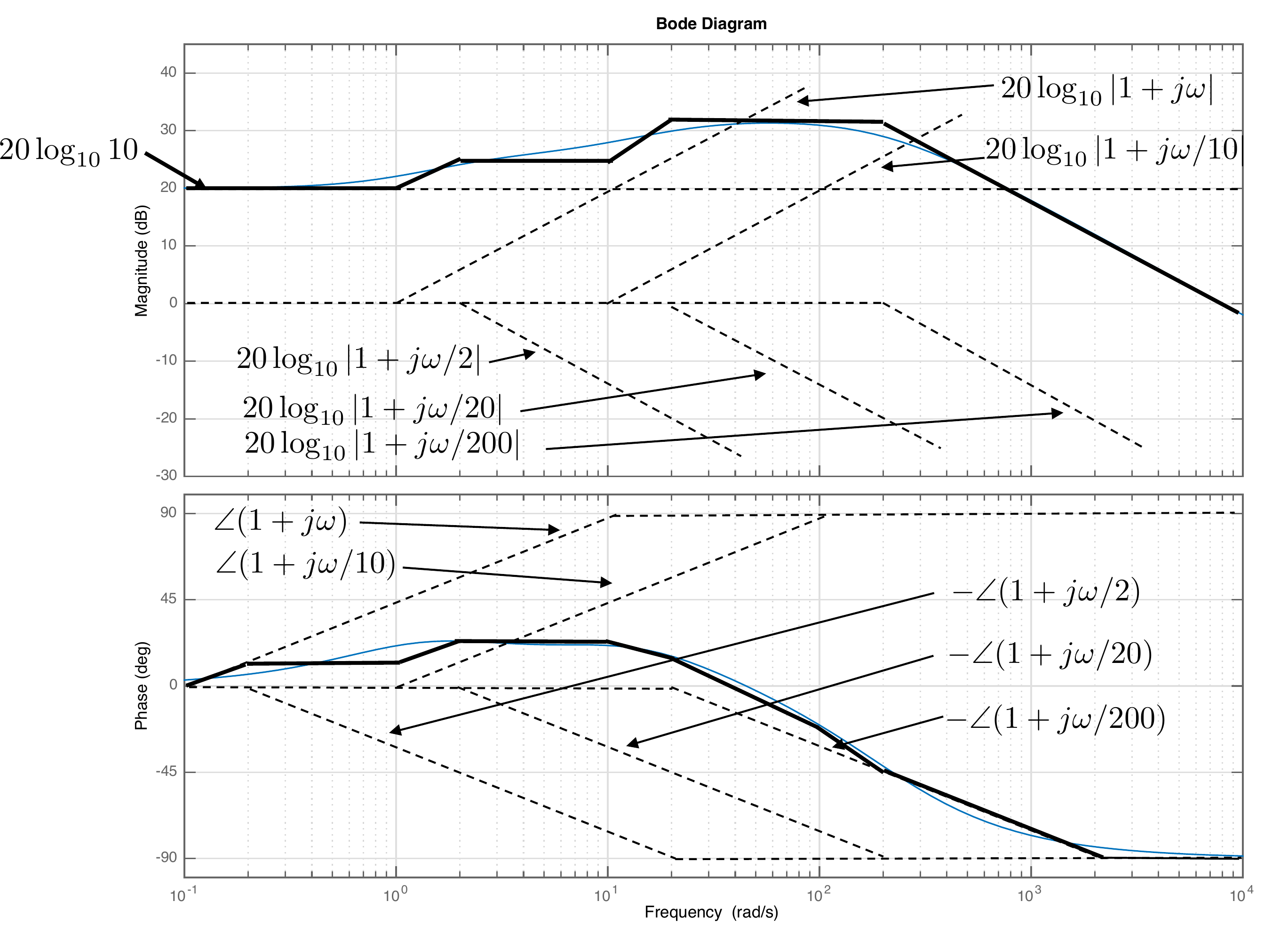
Find the straight-line approximation for the Bode plot of the
transfer function \[\tag{15.12}
H(s) = \frac{8000(s+1)(s+10)}{(s+2)(s+20)(s+200)}.\] In Bode
canonical form we have \[\begin{aligned}
H(j\omega) &= \frac{8000\cdot 10}{2\cdot 20\cdot
200}\frac{(1+j\omega)(1+j\frac{\omega}{10})}
{(1+j\frac{\omega}{2})(1+j\frac{\omega}{20})(1+j\frac{\omega}{200})} \\
&= 10\frac{(1+j\omega)(1+j\frac{\omega}{10})}
{(1+j\frac{\omega}{2})(1+j\frac{\omega}{20})(1+j\frac{\omega}{200})}.
\end{aligned}\] Therefore \[\begin{gathered}
20\log_{10}\left|H(j\omega)\right|=
20\log_{10} 10 +
20\log_{10}\left|1+j\omega\right| + \\
20\log_{10}\left|1+j\frac{\omega}{10}\right|
-20\log_{10}\left|1+j\frac{\omega}{2}\right| \\
-20\log_{10}\left|1+j\frac{\omega}{20}\right|
-20\log_{10}\left|1+j\frac{\omega}{200}\right|.
\end{gathered}\] Therefore, the Bode plot for magnitude will be
the graphical addition of a constant gain, two zeros, and three poles.
Similarly, the phase is given by \[\begin{gathered}
\angle H(j\omega) =
\angle 10
+ \angle (1+j\omega)
+ \angle (1+j\frac{\omega}{10}) \\
- \angle (1+j\frac{\omega}{2})
- \angle (1+j\frac{\omega}{20})
- \angle (1+j\frac{\omega}{200}).
\end{gathered}\] The straight-line approximation and the Bode
plot generated by MATLAB are shown in
Fig.15.11.
Figure 15.11. Bode plot for the transfer function given
in Equation 15.12.
Chapter 15 interactive figure
Build worked examples term by term
Use this review figure to build each worked example the same way as
Example 15.1.4: choose the factors, predict the final high-frequency
behavior, then compare the individual straight-line terms, their
cumulative approximation, and the exact full response.
Interactive Figure 15.I6. The gray curves
show active individual terms, the black dashed curve shows their
cumulative straight-line approximation, and the colored curve shows the
exact full response.
Draw by hand the Bode plot of the single-link robot arm from torque
\(\tilde{\tau}\) to angle \(\tilde{\theta}\) given that the equilibrium
angle is \(\theta_e=0\). Use the
bode command (from MATLAB or Python) and compare your
results.
Design Study A guided exercise
Build the arm Bode plot
Decompose the arm transfer
function into gain, integrator, and first-order pole terms.
Use the plotted response to connect the
gain, integrator, and pole terms to the magnitude slope and phase
trend.
Step 1.
Bode building blocks
Show solution for Step
1
Answer: The arm plant has one
integrator and one real pole from the damping term.
Step 2.
Asymptotic slopes
Show solution for Step
2
Answer: The integrator gives
\(-20\) dB/decade, and the real
pole adds another \(-20\) dB/decade
after its break frequency.
Step 3.
Phase trend
Show solution for Step
3
Answer: The integrator
contributes \(-90^\circ\); the
additional pole drives the phase toward \(-180^\circ\).
Pseudocode
The complete solution includes Bode-plot
generation code. Before opening it, outline how you would define the
transfer function, compute the frequency response, and plot magnitude
and phase.
This
prompt is ungraded. It is intended to connect the Bode construction to
the implementation code in the complete solution.
Complete solution
From HW 3.1.8, the transfer
function for the single-link robot arm is \[\tag{15.14}
P(s) = \frac{3/m\ell^2}{s(s+3b/m\ell^2)} =
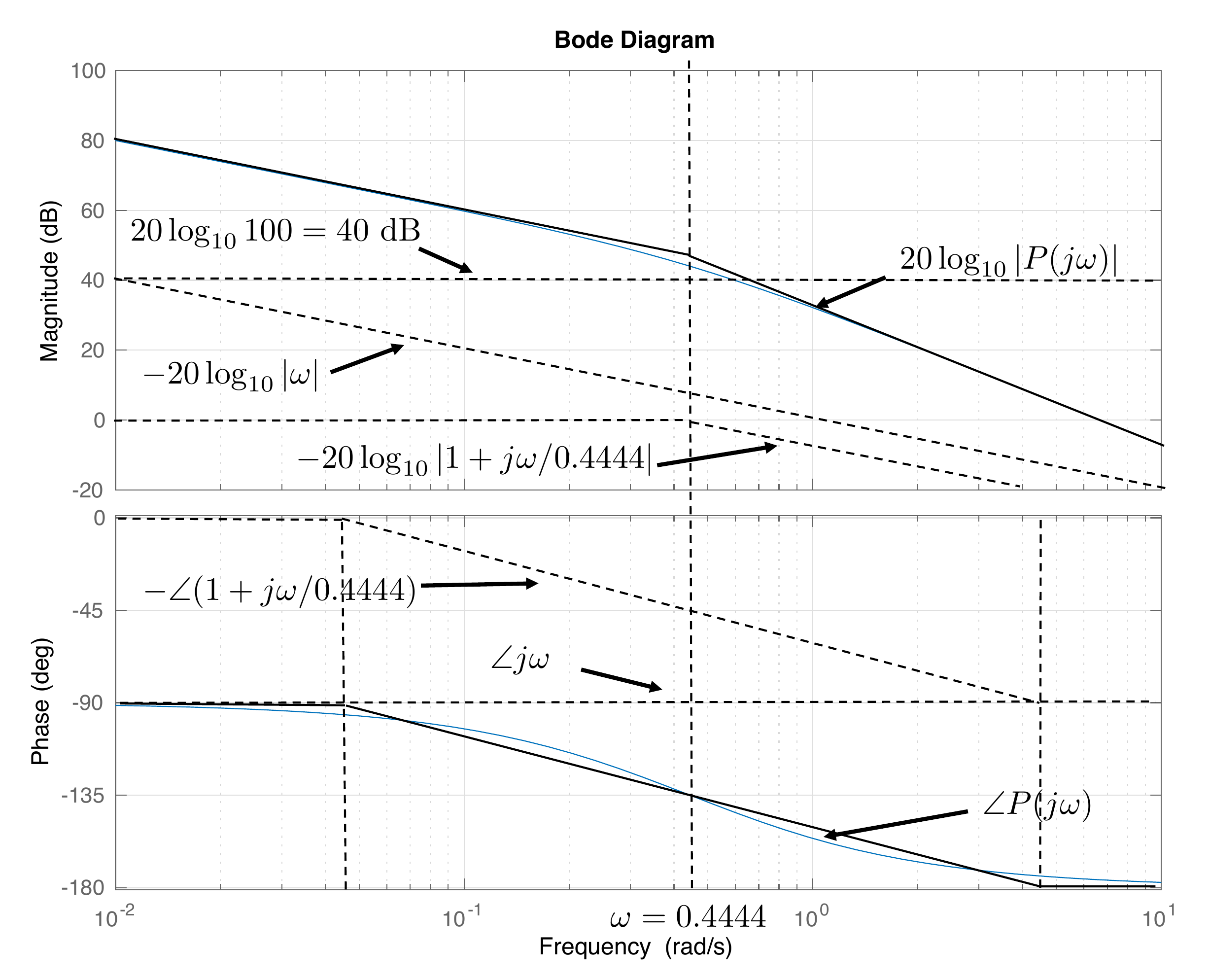
\frac{44.44}{s(s+0.4444)}.\] In Bode canonical form we have \[P(j\omega) =
\frac{100}{(j\omega)(1+j\frac{\omega}{0.4444})}\]
Therefore \begin{gather}
\tag{15.15}
20\log_{10}\left|P(j\omega)\right|=
20\log_{10} 100 \\
-20\log_{10}\left|j\omega\right|
-20\log_{10}\left|1+j\frac{\omega}{0.4444}\right|.
\end{gather} Therefore, the Bode plot for magnitude will be
the graphical addition of a constant gain, an integrator, and a pole.
Similarly, the phase is given by \[\angle
P(j\omega) =
\angle 100
- \angle (j\omega)
- \angle (1+j\frac{\omega}{0.4444}).\]
Figure 15.12. Bode plot for the transfer function given
in Equation 15.14.
Python commands to generate the Bode plots are:
# 3rd-partyimport control as cntimport matplotlib.pyplot as plt# local (controlbook)import case_studies.A_arm.params as Puse_dB =Falseplant = cnt.tf(P.tf_num, P.tf_den)if__name__=="__main__": cnt.bode( plant, dB=use_dB, label="P(s)", legend_loc="best", title="HW 15 Bode Plots: Robot Arm", ) plt.show()
(a) Draw by hand the Bode plot of the inner loop transfer function from
force \(F\) to angle \(\theta\) for the inverted pendulum. Use the
bode command (from MATLAB or Python) and compare your
results.
(b) Draw by hand the Bode plot of the outer loop transfer function from
angle \(\theta\) to position \(z\) for the inverted pendulum. Use the
bode (from MATLAB or Python) command and compare your
results.
Design
Study B guided exercise
Decompose the pendulum Bode
plots
Classify the inner and outer loop transfer-function
factors.
The inner loop includes both a
left-half-plane pole and a right-half-plane pole.
Step 1.
Inner-loop factors
Show
solution for Step 1
Answer: The
inner plant has one LHP pole and one RHP pole.
Step 2.
Outer-loop factors
Show
solution for Step 2
Answer: The
outer plant has two integrators and one LHP/RHP zero
pair.
Step 3.
Comparison method
Show
solution for Step 3
Answer: The
hand sketch is compared against a computed Bode plot.
Pseudocode
The complete solution computes separate
inner-loop and outer-loop Bode plots. Before opening it, outline each
component separately.
These prompts are ungraded. They are
intended to connect the derivation to the implementation code in the
complete solution.
Complete solution
From HW 3.2.8, the transfer
function for the inner loop of the inverted pendulum is \[\tag{15.16}
%
%
P_{in}(s) = \frac{\frac{-1}{(m_1 \frac{\ell}{6}+ m_2 \frac{2
\ell}{3})}}{s^2-\frac{(m_1+m_2)g}{(m_1 \frac{\ell}{6}+ m_2 \frac{2
\ell}{3})}} =
\frac{-1.42}{s^2 - 17.29} = \frac{-1.42}{(s+4.16)(s-4.16)}. %\]
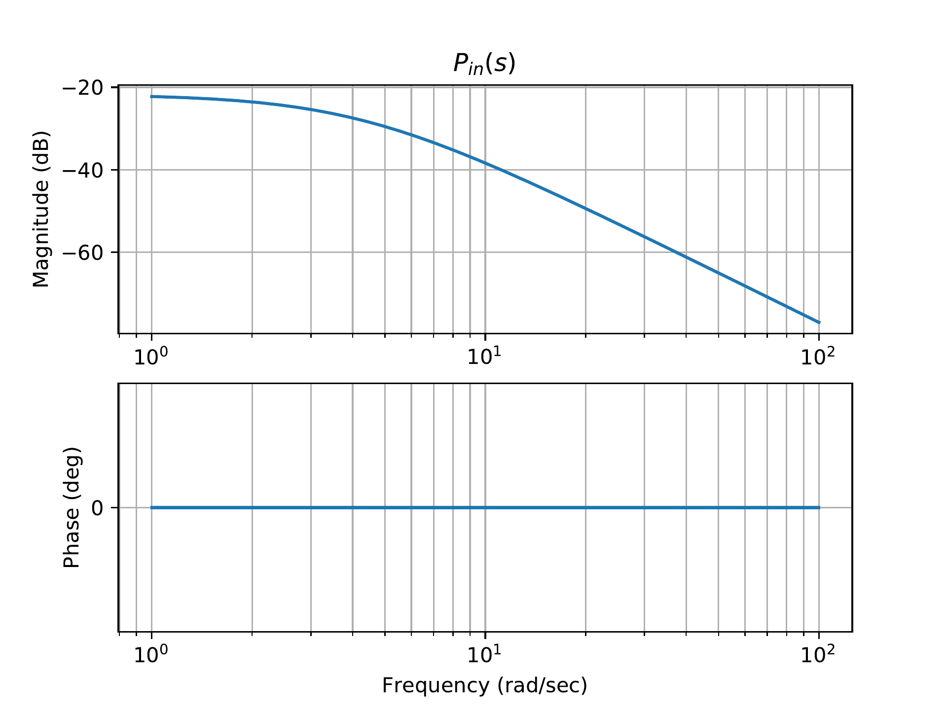
In Bode canonical form we have \[P_{in}(j\omega) =
\frac{0.0659}{(1+j\frac{\omega}{4.16})(1-j\frac{\omega}{4.16})}\]
Therefore \begin{gather}
\tag{15.17}
20\log_{10}\left|P_{in}(j\omega)\right|=
20\log_{10} 0.0659 \\
-20\log_{10}\left|1+j\frac{\omega}{4.16}\right|
-20\log_{10}\left|1-j\frac{\omega}{4.16}\right|.
\end{gather} Therefore, the Bode magnitude plot will be the
graphical addition of a constant gain, a right-half-plane pole, and a
left-half-plane pole. Similarly, the phase is given by \[\angle P_{in}(j\omega) =
\angle 0.0816
- \angle (1+j\frac{\omega}{4.16})
- \angle (1-j\frac{\omega}{4.16}).\] The Bode plot generated
by Python is shown in Fig.15.13.
Figure 15.13. Bode plot for the transfer function given
in Equation 15.17.
From HW 3.2.8, the transfer
function for the outer loop of the inverted pendulum is \[\tag{15.18}
P_{out}(s) = -\frac{\frac{2 \ell}{3} s^2 - g}{s^2} =
-\frac{\frac{2}{3}\ell (s^2 - \frac{g}{\ell}\frac{3}{2})}{s^2} =
-\frac{\frac{2}{3}(s-3.83)(s+3.83)}{s^2}.\] In Bode canonical
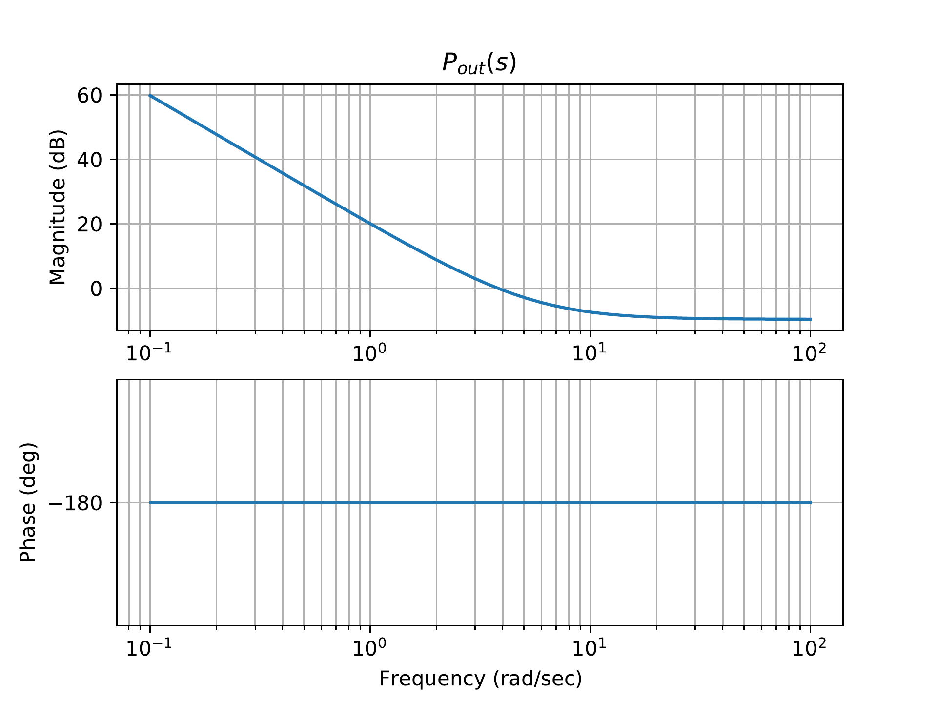
form we have \[P_{out}(j\omega) =
\frac{0.174(j\omega/3.83+1)(-j\omega/3.83+1)}{(j\omega)^2}.\]
Therefore \begin{gather}
\tag{15.19}
20\log_{10}\left|P_{out}(j\omega)\right|= \\
20\log_{10} 0.174
+ 20\log_{10}\left|1+j\frac{\omega}{3.83}\right| \\
+ 20\log_{10}\left|1+j\frac{\omega}{-3.83}\right|
-20\log_{10}\left|\omega\right|^2.
\end{gather} Similarly, the phase is given by \[\angle P_{out}(j\omega) =
\angle 0.174
+ \angle (1+j\frac{\omega}{3.83})
+ \angle (1-j\frac{\omega}{3.83})
- \angle (j\omega)
- \angle (j\omega).\]
The Bode plot generated by Python is shown in
Fig.15.14.
Figure 15.14. Bode plot for the transfer function given
in Equation 15.19.
Python code to generate Bode plots for the previous two figures is as
follows:
# 3rd-partyimport control as cntimport matplotlib.pyplot as plt# local (controlbook)import case_studies.B_pendulum.params as Puse_dB =Falseplant_inner = cnt.tf(P.tf_inner_num, P.tf_inner_den)plant_outer = cnt.tf(P.tf_outer_num, P.tf_outer_den)if__name__=="__main__": cnt.bode( [plant_inner, plant_outer], dB=use_dB, label=[r"$P_{inner}(s)$", "$P_{outer}(s)$"], legend_loc="best", title="HW 15 Bode Plots: Pendulum on a Cart", ) plt.show()
(a) Draw by hand the Bode plot of the inner loop transfer function from
torque \(\tau\) to angle \(\theta\) for the satellite attitude
problem. Use the bode command (from MATLAB or Python) and
compare your results.
(b) Draw by hand the Bode plot of the outer loop transfer function from body
angle \(\theta\) to panel angle \(\phi\) for the satellite attitude problem.
Use the bode command (from Python or MATLAB) and compare
your results.
Design Study C guided exercise
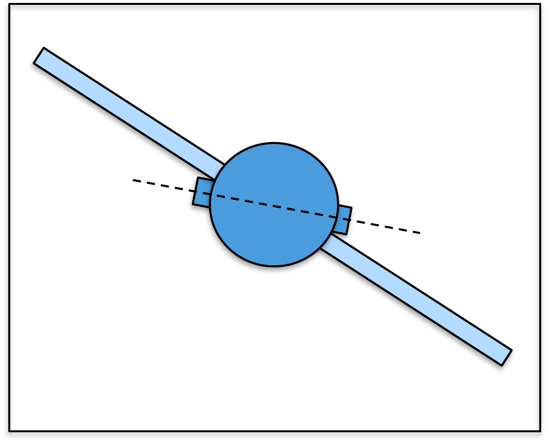
Build satellite Bode plots
The inner loop behaves like
two integrators; the outer loop contains a lightly damped flexible
mode.
Step 1. Inner plant structure
Show
solution for Step 1
Answer:
\(P_{in}(s)=1/(6s^2)\), with slope \(-40\) dB/dec and phase
\(-180^\circ\).
Step 2. Outer
plant structure
Show solution for Step
2
Answer: \(P_{out}(s)\) has a
numerator zero and a lightly damped flexible-mode pole
pair.
Step 3. Physical interpretation
Show solution for Step
3
Answer: Aggressive designs can
excite the flexible panel mode, visible as oscillation in
\(\phi-\theta\).
Complete solution
From HW 3.3.8, the transfer
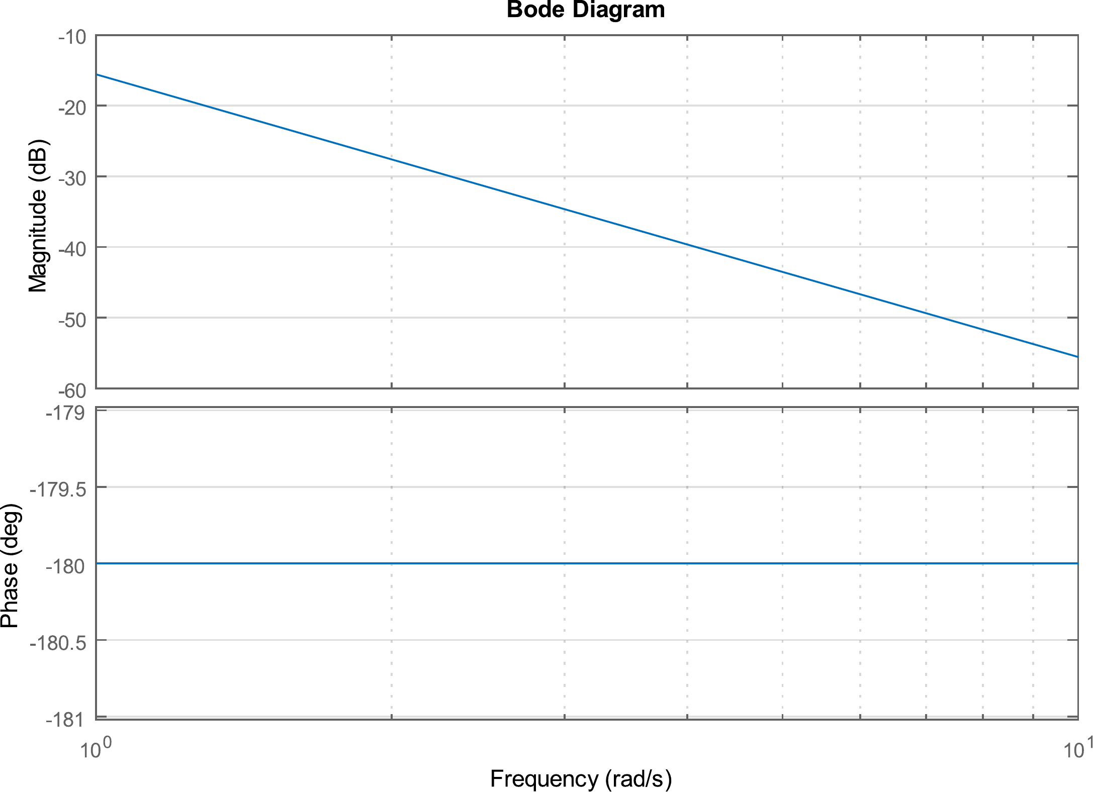
function for the inner loop of the satellite attitude problem is \[\tag{15.20}
%
%
P_{in}(s) = \frac{1}{(J_s + J_p)s^2} =
\frac{1}{6s^2}.\] In Bode canonical form we have \[%
P_{in}(j\omega) = \frac{1}{6}\frac{1}{(j\omega)(j\omega)}.\]
Therefore, \[\tag{15.21}
%
%
%
20\log_{10}\left|P_{in}(j\omega)\right|=
20\log_{10}
1/6-20\log_{10}\left|\omega\right|-20\log_{10}\left|\omega\right|\]
Therefore, the Bode plot for magnitude will be the graphical addition of
a constant gain and two straight lines passing through the 0 dB line at
\(\omega = 1\) with a slope of -20
dB/decade. Similarly, the phase is given by \[%
%
%
\angle P_{in}(j\omega) =
\angle 1/6
- \angle j\omega - \angle j\omega.\] The Bode plot generated by
MATLAB is shown in Fig.15.15. As can be seen from
the figure, the straight-line approximation corresponds directly with
the Bode plot in this case.
Figure 15.15. Bode plot for the transfer function given
in Equation 15.21.
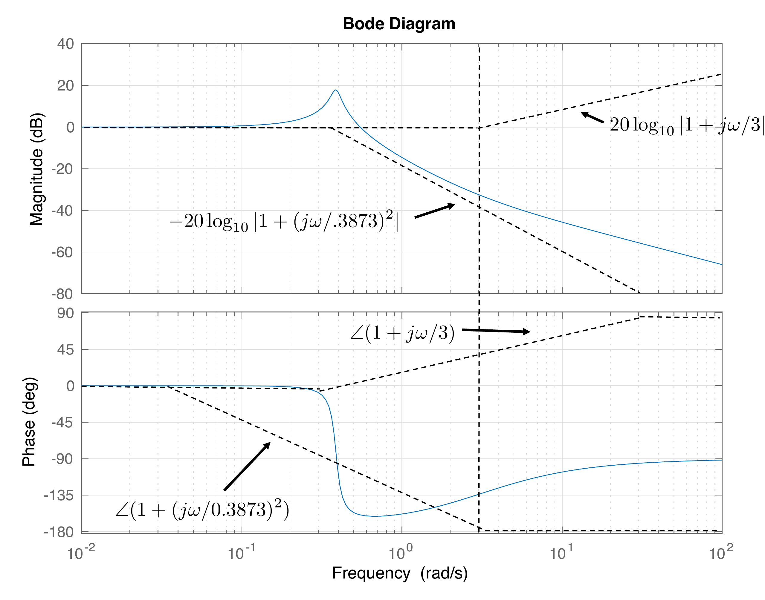
From HW 3.3.8, the transfer
function for the outer loop of the satellite is \[\tag{15.22}
P_{out}(s) =
\frac{\frac{b}{J_p}s+\frac{k}{J_p}}{s^2+\frac{b}{J_p}s+\frac{k}{J_p}} =
\frac{0.05s + 0.15}{s^2+0.05s+0.15}.\] In Bode canonical form we
have \[P_{out}(j\omega) =
\frac{1+j\frac{\omega}{3}}{1+j\frac{\omega}{3} +
\left(j\frac{\omega}{0.3873}\right)^2}\] Therefore \begin{gather}
\tag{15.23}
20\log_{10}\left|P_{out}(j\omega)\right|=
20\log_{10} \left|1+j\omega/3\right| \\
-20\log_{10}\left|1+j\omega/3 +
\left(j\frac{\omega}{0.3873}\right)^2\right|
\end{gather} Therefore, the Bode plot for magnitude will be
the graphical addition of a zero, and a complex pole. Similarly, the
phase is given by \[\angle P_{out}(j\omega) =
\angle \left(1+j\omega/3\right)
- \angle \left(1+j\omega/3 +
\left(j\frac{\omega}{0.3873}\right)^2\right).\] The straight-line
approximation and the Bode plot generated by MATLAB are shown in
Fig.15.16.
Figure 15.16. Bode plot for the transfer function given
in Equation 15.23.
The Python code to generate similar Bode plots is
# 3rd-partyimport control as cntimport matplotlib.pyplot as plt# local (controlbook)import case_studies.C_satellite.params as Puse_dB =Falseplant_inner = cnt.tf(P.tf_inner_num, P.tf_inner_den)plant_outer = cnt.tf(P.tf_outer_num, P.tf_outer_den)if__name__=="__main__": cnt.bode( [plant_inner, plant_outer], dB=use_dB, label=[r"$P_{inner}(s)$", "$P_{outer}(s)$"], legend_loc="best", title="HW 15 Bode Plots: Satellite", ) plt.show()
15.5 Interactive Frequency-Response
Check
Chapter 15 activity
Complex response readout
Move the real and imaginary parts of
H(jω). The readout connects
rectangular form, magnitude, phase, and dB magnitude, which are the same
quantities used to build Bode plots.
Figure 1.5. The sliders move the
complex frequency-response vector and change its magnitude and
phase.
Rectangular form
Magnitude
Phase
Magnitude in dB
Coding-lab preparation: evaluating a frequency response means
substituting s = jw, then computing magnitude, phase, and dB values over
a frequency grid.
15.6 Coding Lab: Frequency Response
Evaluation
Objective: evaluate a transfer function on the
imaginary axis and compute Bode magnitude and phase.
Evaluation criteria: the lab checks complex
substitution at s = jw, vectorized array output, magnitude in dB, and
phase in degrees.
Frequency response is
found by evaluating a transfer function at:
Q2. Pole
slope
A pole typically changes the
high-frequency magnitude slope by:
Q3. Complex magnitude
Enter the magnitude of the complex number 3 + j4.
Show solution
Answer: 5 because sqrt(3^2 + 4^2) = 5.
Q4. dB conversion
Enter 20 log10(0.1) in dB.
Show solution
Answer: -20 dB because log10(0.1) = -1.
Q5.
Sinusoidal steady-state output
For
stable G(s) = 3/(s + 4) and input u(t) = 2 sin(t), which steady-state
output is closest?
Q6. Complex substitution
What substitution converts a transfer function
G(s) into its frequency response?
Q7. Net Bode slope
At frequencies well above both break frequencies,
what net magnitude-slope change comes from one pole and one zero?
Q8. dB conversion
Which dB value is closest to a magnitude ratio of
0.5?
Q9. Phase-lead interpretation
Which statement best describes the effect of
increasing the lead parameter M in a phase-lead block?
15.8 Notes and References
A good introduction to frequency response for linear time-invariant
system is [16]. A good overview of the Bode plot and straight-line
approximations to the Bode plot is contained in [4] and many other
introductory textbooks on feedback control.